fit_INST_ARL2_part1.m
Fit the INST model (aka protoanchor) to the group ARL2 profiles of the Fdbk1 Experiment. The goal is to show that this model cannot fit these data very well.
The main tool is .../work/models/protoanchor/protoanchor_ARL2.m
File: work/CMUExper/fdbk1/data/fit_INST_ARL2_part1.m
Date: 2007-08-16
Alexander Petrov, http://alexpetrov.com
Contents
- Load the data
- Collapse across groups
- Fit INST on the same stimulus sequences, 11 per group
- Search parameters
- "Chance event" sets
- Cutoff parameter grid
- Main work
- Plot the SSE
- Plot the memory noise parameter
- Plot the temperature parameter
- Interim conclusion
- Generate and ARL2 profiles with these parameters
- Plot the "optimal" ARL2 profiles
- Define Assimilation := ARL(N)-ARL(P) and plot Assim profile
- Clean up
Load the data
clear all
cd(fullfile(work_pathstr,'CMUExper','fdbk1','data')) ;
load('S2.mat') ;
ARL2 = [S2(:).ARL2] ;    % 9x55
gr=[S2(:).group]' ;
ugr = unique(gr) ;
N_groups = length(ugr) ;
ugr_descr = {'U1' 'L1' 'H1', 'L2' 'H2' } ;   % [1 2 3, 5 6]
Collapse across groups
grARL2 = zeros(size(ARL2,1),N_groups) ;   % 9x5
gr_idx = cell(1,N_groups) ;
for k = 1:N_groups
    gr_idx{k} = find(gr==ugr(k))' ;
    grARL2(:,k) = mean(ARL2(:,gr_idx{k}),2) ;
end
grARL2
grARL2 =
    4.3358    4.1354    4.2075    4.1789    4.2197
    4.0525    4.0594    4.1666    4.6730    4.1990
    4.1878    3.9444    4.2666    4.7687    4.0890
    4.4236    4.4190    4.4370    3.9850    4.3336
    4.3422    4.2662    4.4461    3.9343    4.3488
    4.2404    3.8147    4.4136    4.1016    4.2765
    4.0962    3.7438    4.3909    4.2058    4.4644
    4.2742    3.9327    4.3790    3.8922    4.3864
    4.3494    3.6773    4.5247    3.7794    4.3898
Fit INST on the same stimulus sequences, 11 per group
stim = [S2(:).dist] ;   % 476x55
fdbk = [S2(:).fdbk] ;
Search parameters
These control the optimizer via the PARAMSEARCH Toolbox. FMINCON is used (instead of LSQNONLIN) because experimental fits of synthetic ARL2 profiles showed that it works somewhat better in our setting. Still, the cutoff parameters cannot be fitted with these methods, probably because the error derivative is not continuous w.r.t. the cutoffs. The plan is to explore the two cutoff parameters on a grid, while optimising w.r.t three others: mem_k, temper, and hist. The perceptual noise is fixed a priori to perc_k=.040. The history weight parameter is poorly determined by the data. Therefore, at first we fix it at H=.040 and do a grid search on the cutoff parameters. When we narrow down the relevant region of the parameter space, we will revisit H again.
fminconp = 1 ;
flags = [0 1 1 0 0 0 0 0] ;   % [perc_k mem_k temper hist cutoff xx xx c_ratio]
Sparams = protoanchor_search_params(flags,fminconp) ;
optns = optimset(Sparams.optns,'TolX',1e-2,'Display','off') ;
Sparams.optns = optns ;
Sparams.target_vals = grARL2
H = .040 ; Sparams.params.history = H ;   % for the time being
Sparams.params
Sparams =
     model_name: 'protoanchor_ARL2'
         params: [1x1 struct]
      p2v_templ: {'VAL = PARAMS.mem_k * 10 ;'  'VAL = PARAMS.temper * 10 ;'}
      v2p_templ: {'PARAMS.mem_k = VAL / 10 ;'  'PARAMS.temper = VAL / 10 ;'}
         bounds: [2x2 double]
     ARL_params: [1x1 struct]
    funfun_name: 'fmincon'
          optns: [1x1 struct]
     lsfun_name: 'sumsqerr'
    target_vals: [9x5 double]
ans =
        scale: 'LINEAR'
        N_cat: 7
      SM_conv: 1.0000e-03
       cat_sz: 0.0400
       perc_k: 0.0400
        mem_k: 0.0700
        avail: [7x1 double]
    instances: [7x3 double]
      cutoffs: [-2.4000 -0.8000 0.7200 2.1600]
       temper: 0.0400
      history: 0.0400
        alpha: 0.3000
        decay: 0.5000
          ITI: 4
"Chance event" sets
The model is fitted using the deterministic version PROTOANCHOR_CHEV that uses previously cached values of all randomly generated values. More than one such "chev" sets is used to evaluate its impact on the fit.
N_chevs = 2 ;

% Pack into "model data" structures suitable for passing as arguments.
Mdata = cell(1,N_chevs) ;
for k = 1:N_chevs
    Mdata{k}.stim = stim ;
    Mdata{k}.fdbk = fdbk ;
    Mdata{k}.group_idx = gr_idx ;
    %Mdata{k}.params = Sparams.params ;    % will be set by SUMSQERR
    Mdata{k}.chev = make_protoanchor_chev(size(stim,1),size(stim,2)) ;
    Mdata{k}.ARL_params = Sparams.ARL_params ;
end
Cutoff parameter grid
cutoff_levels = [.50 .55 .60 .65 .70 .80 .90 1.00]' ;  % c- in categ_sz units
N_cutoff_levels = length(cutoff_levels) ;
c_ratio_levels = [.5 .6 .7 .8 .9] ;          % c-/c+ ratio
N_c_ratio_levels = length(c_ratio_levels) ;
Main work
A grid search over 5x3x2 cells takes five hours on a fast machine. Therefore, the results will only be computed once and cached to disk.
fname = 'grid_search_INST_ARL2_part1.mat' ;
if (file_exists(fname))
    load(fname) ;
else
  grid_SSE = zeros([N_cutoff_levels,N_c_ratio_levels,N_chevs]) ;
  grid_optX = cell([N_cutoff_levels,N_c_ratio_levels,N_chevs]) ;
  grid_det = cell([N_cutoff_levels,N_c_ratio_levels,N_chevs]) ;
  tic
  for k1 = 1:N_cutoff_levels
      c = cutoff_levels(k1) ;
      fprintf('\n cutoff %4.2f: ',c) ;
      for k2 = 1:N_c_ratio_levels
          cr = c_ratio_levels(k2) ;
          cutoffs = c .* [-3 -1 cr 3*cr] ;
          Sparams.params.cutoffs = cutoffs ;
          for k = 1:N_chevs
              [par,SSE,optX,det] = paramsearch(Mdata{k},Sparams) ;  % <-- Sic!
              grid_SSE(k1,k2,k) = SSE ;
              grid_optX{k1,k2,k} = optX ;
              grid_det{k1,k2,k} = det ;
              fprintf('%5.3f ',SSE) ;
              save(fname,'grid_SSE','grid_optX','grid_det','Sparams',...
                   'cutoff_levels','c_ratio_levels') ;
          end
          fprintf(', ') ;
      end
  end
  fprintf('\n') ;
  toc
end % if file_exists ...
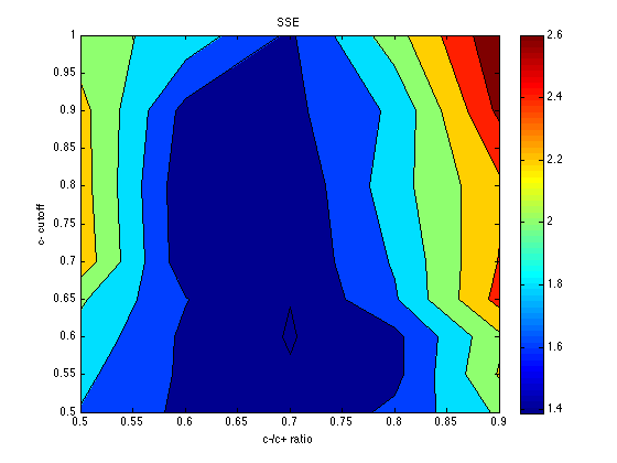
Plot the SSE
SSE = mean(grid_SSE,3)   % average across the chev's
[X,Y] = meshgrid(c_ratio_levels,cutoff_levels) ;
contourf(X,Y,SSE) ; colorbar ; title('SSE') ;
xlabel('c-/c+ ratio') ; ylabel('c- cutoff') ;
SSE =
    1.7888    1.5530    1.4217    1.6504    2.0318
    1.8492    1.5656    1.4132    1.5419    2.2204
    1.9386    1.5639    1.3889    1.5422    2.1584
    2.0268    1.6076    1.4028    1.7743    2.4702
    2.3314    1.4707    1.4331    1.8232    2.4112
    2.2935    1.4553    1.4324    1.9165    2.3614
    2.2761    1.5362    1.5492    1.8376    2.6434
    2.0776    1.9287    1.5657    2.1168    2.7561
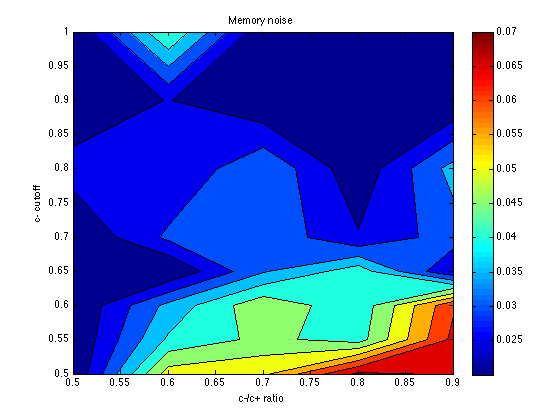
Plot the memory noise parameter
mem_k = zeros(size(grid_optX)) ;
temper = zeros(size(grid_optX)) ;
for k1 = 1:N_cutoff_levels
    for k2 = 1:N_c_ratio_levels
        for k = 1:N_chevs
            mem_k(k1,k2,k) = grid_optX{k1,k2,k}(1) / 10 ;
            temper(k1,k2,k) = grid_optX{k1,k2,k}(2) / 10 ;
        end
    end
end

mem_k = mean(mem_k,3)
contourf(X,Y,mem_k) ; colorbar ; title('Memory noise') ;
xlabel('c-/c+ ratio') ; ylabel('c- cutoff') ;
mem_k =
    0.0200    0.0527    0.0542    0.0714    0.0696
    0.0200    0.0408    0.0464    0.0426    0.0664
    0.0200    0.0365    0.0489    0.0412    0.0643
    0.0200    0.0200    0.0345    0.0428    0.0250
    0.0200    0.0310    0.0340    0.0254    0.0326
    0.0273    0.0251    0.0346    0.0213    0.0368
    0.0200    0.0252    0.0201    0.0240    0.0202
    0.0200    0.0452    0.0209    0.0200    0.0200
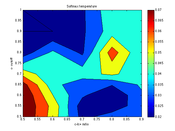
Plot the temperature parameter
temper = mean(temper,3)
contourf(X,Y,temper) ; colorbar ; title('Softmax temperature') ;
xlabel('c-/c+ ratio') ; ylabel('c- cutoff') ;
temper =
    0.0800    0.0558    0.0266    0.0355    0.0329
    0.0800    0.0569    0.0246    0.0226    0.0368
    0.0800    0.0504    0.0317    0.0205    0.0384
    0.0744    0.0441    0.0319    0.0306    0.0416
    0.0567    0.0418    0.0462    0.0521    0.0429
    0.0240    0.0420    0.0280    0.0653    0.0406
    0.0200    0.0200    0.0281    0.0451    0.0456
    0.0200    0.0274    0.0281    0.0475    0.0438
Interim conclusion
The optimum seems to be located for: cutoff = .60 category_sz units cutoff_ratio = 0.7 Thus, cutoffs = .60 .* [-3 -1 .7 3*.7] = [-1.8 -.6 .42 1.26]. Memory noise seems to be about mem_k = .050 (or less), which is less than the default (.070) in PetrovAnderson05. The temperature parameter seems poorly determined, but temper = .040 seems a reasonable starting point for subsequent explorations. This is again less than the default (.050) in PetrovAnderson05.
optX = [.040 .050].*10 ;
Mparams = vector2params(optX,Sparams.params,Sparams.v2p_templ) ;
Mparams.cutoffs = .60 .* [-3 -1 .7 3*.7]
Mparams =
        scale: 'LINEAR'
        N_cat: 7
      SM_conv: 1.0000e-03
       cat_sz: 0.0400
       perc_k: 0.0400
        mem_k: 0.0400
        avail: [7x1 double]
    instances: [7x3 double]
      cutoffs: [-1.8000 -0.6000 0.4200 1.2600]
       temper: 0.0500
      history: 0.0400
        alpha: 0.3000
        decay: 0.5000
          ITI: 4
Generate and ARL2 profiles with these parameters
for k = 1:N_chevs
    Mdata{k}.params = Mparams ;
    opt_grARL2(:,:,k) = protoanchor_ARL2(Mdata{k}) ;
end
opt_grARL2 = mean(opt_grARL2,3) ;
[grARL2 opt_grARL2]
opt_SSE = (grARL2-opt_grARL2) ;
opt_SSE = sum(opt_SSE(:).^2)
ans =
    4.3358    4.1354    4.2075    4.1789    4.2197    4.1094    4.0922    4.1151    4.1485    4.1193
    4.0525    4.0594    4.1666    4.6730    4.1990    4.1061    4.0228    4.2128    4.1561    4.2446
    4.1878    3.9444    4.2666    4.7687    4.0890    4.1031    3.9662    4.2516    4.2408    4.3463
    4.4236    4.4190    4.4370    3.9850    4.3336    4.1511    4.0063    4.3381    4.1448    4.3778
    4.3422    4.2662    4.4461    3.9343    4.3488    4.1914    4.0867    4.4002    4.0964    4.3611
    4.2404    3.8147    4.4136    4.1016    4.2765    4.1994    4.0561    4.3598    4.1028    4.3661
    4.0962    3.7438    4.3909    4.2058    4.4644    4.1582    4.0096    4.3427    4.1044    4.4449
    4.2742    3.9327    4.3790    3.8922    4.3864    4.1771    4.0186    4.3711    4.0743    4.4204
    4.3494    3.6773    4.5247    3.7794    4.3898    4.2143    4.0323    4.4161    4.0481    4.4310
opt_SSE =
    1.5061
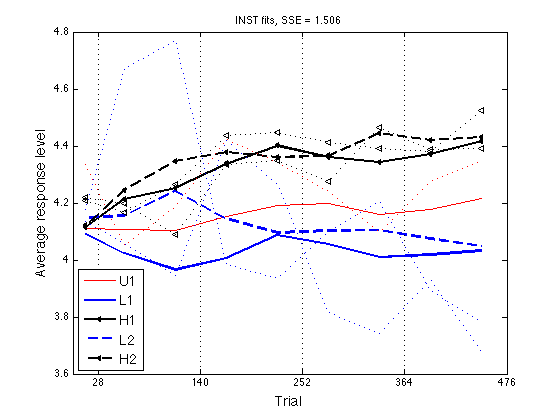
Plot the "optimal" ARL2 profiles
ls = {'r-' 'b-' 'k<-' 'b--' 'k<--'} ;   % group line styles
lw = [1 2 2  2 2] ;                     % group line widths
els  = {'r:' 'b:' 'k<:' 'b:' 'k<:'} ;   % empirical-data line styles

x2 = [14 , 56:56:448]' ;
xtick = [28 , 140:112:476] ;
ytick = [3.6:.2:4.8] ;
ax = [0 476 3.6 4.8] ;

clf ; hold on ;
for k = 1:N_groups
    hh = plot(x2,opt_grARL2(:,k),ls{k}) ;
    set(hh,'LineWidth',lw(k),'MarkerSize',4) ;
end
for k = 1:N_groups
    plot(x2,grARL2(:,k),els{k}) ;
end
hold off ; box on ;
axis(ax) ; set(gca,'xtick',xtick,'ytick',ytick,'xgrid','on') ;
hh = xlabel('Trial') ; set(hh,'FontSize',14) ;
hh = ylabel('Average response level') ; set(hh,'FontSize',14) ;
hh = legend('U1','L1','H1','L2','H2',3) ; set(hh,'FontSize',14) ;
title(sprintf('INST fits, SSE = %.3f',opt_SSE)) ;
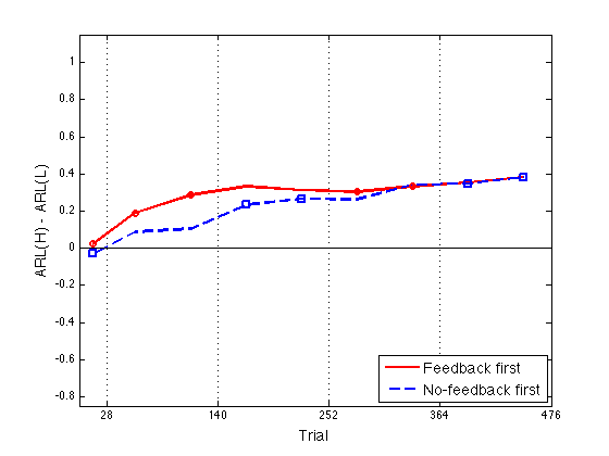
Define Assimilation := ARL(N)-ARL(P) and plot Assim profile
See .../CMUExper/fdbk1/data/empir_ARL2_profile.m
%Assim = grARL2(:,[3 find(ugr==6)]) - grARL2(:,[2 find(ugr==5)])
opt_Assim = opt_grARL2(:,[3 find(ugr==6)]) - opt_grARL2(:,[2 find(ugr==5)])

ax = [0 476 -0.85 1.15] ;
ytick1 = [-.8:.2:1] ;
idx1 = [1 2 3 6 7] ;    % feedback blocks for the feedback-first groups
idx2 = [1 4 5 8 9] ;    % feedback blocks for the no-feedback-first grps

clf ;
hh = plot(x2,opt_Assim(:,1),'r-',x2,opt_Assim(:,2),'b--',...
          x2(idx1),opt_Assim(idx1,1),'ro',x2(idx2),opt_Assim(idx2,2),'bs') ;
    set(hh,'LineWidth',2) ;
    axis(ax) ;
    hh=refline(0,0) ;
    set(hh,'Color','k','LineStyle','-','LineWidth',1) ;
box on ;
axis(ax) ; set(gca,'xtick',xtick,'ytick',ytick1,'xgrid','on') ;
hh = xlabel('Trial') ; set(hh,'FontSize',14) ;
hh = ylabel('ARL(H) - ARL(L)') ; set(hh,'FontSize',14) ;
hh = legend('Feedback first','No-feedback first',4) ; set(hh,'FontSize',14) ;

% The fitting effort continues in fit_INST_ARL2_part2.m
opt_Assim =
    0.0230   -0.0292
    0.1900    0.0885
    0.2854    0.1055
    0.3318    0.2329
    0.3135    0.2647
    0.3037    0.2633
    0.3331    0.3405
    0.3525    0.3461
    0.3838    0.3829
Clean up
clear k k1 k2 X Y ax hh ;