MLZ02_dpr_group_fits.m
Nonlinear fits of the group-level d' data from the MLSecond02 experiment
File: work/MLExper/MLSecond02/analysis/MLZ02_dpr_group_fits.m
1.2.1 2010-01-29 AP: test whether Y24 < Y18 for Group 1
1.2.0 2010-01-21 AP: z-tests based on bootstrap estimates of variance
1.1.0 2009-10-09 TH: Added the "new eleven-parameter model"
1.0.0 2009-09-04 AP: Wrote it, based on MLPilot02/anal/dpr_group_fits.m
Contents
- Get started
- Design parameters
- Load the data
- Adjust dprime for sbj 325, Day 3, which is anomalously bad for this sbj.
- Save the adjusted data for future use by MLZ01_dprfit_bootstrap
- Time- and task-related variables -- See MLSecond02_params for details
- Pack the dprime2 data into matrices
- Subtract individual subjects' means to estimate within-sbj variance
- Aggregate the data into 4 group averages
- Plot adprime2 for all 4 groups
- Average REFERENCE DIRECTION out to make two supergroups: First and Second
- Plot adprime2 for the two (super)groups
- Plot easy and hard d' separately
- Prepare to run MLZ02_lsqcurvefit: Saturated model
- Fit the saturated model
- Plot the fit of the saturated model
- Saturated model with common time constants
- Fit the saturated model with common time constants
- Significance test for nested multiple regression models
- Plot the fit of the saturated model with common time constants
- Proportionality between Easy and Hard d'
- Independent-group model with Easy/Hard proportionality
- Fit the independent-group model with Easy/Hard proportionality
- Plot the fit of the independent-group model with Easy/Hard proportionality
- Twelve-parameter model: Common Y1, Y2, Y3
- Fit the twelve-parameter model
- Plot the fit of the twelve-parameter model
- Eleven-parameter model: Common Y18
- Fit the eleven-parameter model
- New Eleven-parameter model: HdGr2Y19==HdGr2Y24
- Fit the New Eleven-parameter model (HdGr2Y19==HdGr2Y24)
- Plot the fit of the New Eleven-parameter model
- Define two specificity indices
- Compute both specificity indices for all regression fits
- Prepare to run MLZ02_dprfit_bootstrap
- Calculate bootstrap samples
- The first "sample" is always the full data set:
- Explore the New 11-parameter model performance
- Explore the parameters of the New 11-parameter model
- z-test for the learning effect
- z-test whether there is more learning in Group 1 than in Group 2
- z-test whether Y24 < Y18 in Group 1
- Descriptive statistics about the tau1-to-tau2 ratio
- Explore 15-parameter model performance
- Explore the parameters of the 15-parameter model
- Explore the raw specificity indices
- Explore the specificity indices under the New 11-parameter model
- Explore the specificity indices under the 15-parameter model
- 2010-01-29
Get started
cd(fullfile(MLSecond02_pathstr,'analysis')) ;
fprintf('\n\nExecuting MLZ02_dpr_group_fits on %s.\n\n',datestr(now)) ;
fprintf('cd %s\n',pwd) ;

clear all ;
Executing MLZ02_dpr_group_fits on 29-Jan-2010 17:44:36.

cd /Users/apetrov/a/r/w/work/MLExper/MLSecond02/analysis
Design parameters
Load them from the code that administered the experiment:
P = MLZ02_params(0) ;
design_params = P.design_params ;

N_sessions = design_params.max_session ;          % 6 sessions
blocks_session = design_params.blocks_session ;   % 8 blocks per session
  % Note: We're going to aggregate blocks two by two below.
  % So, the effective number of blocks per session is 4 rather than 8
blocks2_session = blocks_session / 2 ;
N_blocks = N_sessions * blocks_session ;
N_blocks2 = N_sessions * blocks2_session ;
trials_block = design_params.trials_block ;       % 104 trials per block
trials_block2 = 2*trials_block ;                  % 208 per double-block
N_trials = N_blocks * trials_block ;
group_descr = design_params.group_descr'  %#ok<*NOPTS>
deltas = design_params.deltas ;           % [11 8] = [easy difficult]
group_descr =

    'FirstNeg'
    'SecondNeg'
    'FirstPos'
    'SecondPos'
Load the data
H_filename = fullfile(MLSecond02_pathstr,'data','H.mat') ;
if (exist(H_filename,'file'))
    fprintf('load %s \n\n',H_filename) ;
    load(H_filename) ;
else
    error('Cannot find %s.\n Run MLZ02_plot_dprime to create it if necessary.',...
          H_filename) ;
end

% Make sure all data sets in H are complete
N = [H.N] ;
assert(all(N==N_blocks)) ;
N_sbj = length(H) ;

gr = [H.group] ;
xtab1(gr')
load /Users/apetrov/a/r/w/work/MLExper/MLSecond02/data/H.mat


   Value   Count  Percent  Cum_cnt  Cum_pct
-------------------------------------------
       1       5    25.00        5    25.00
       2       5    25.00       10    50.00
       3       5    25.00       15    75.00
       4       5    25.00       20   100.00
-------------------------------------------
Adjust dprime for sbj 325, Day 3, which is anomalously bad for this sbj.
The constants 0.95, 1.10, 0.60 were chosen by eye to make the corresponding learning curves smooth across Days 2-4. Crit2 and RTs are left alone. Sbj 325 was assigned to Group 3 (FirstPos).
sbj325 = find([H.sbj]==325) ;
day3 = (9:12) ;
H(sbj325).all_dprime2(day3) = H(sbj325).all_dprime2(day3) + 0.95 ;
H(sbj325).easy_dprime2(day3) = H(sbj325).easy_dprime2(day3) + 1.10 ;
H(sbj325).hard_dprime2(day3) = H(sbj325).hard_dprime2(day3) + 0.60 ;
%dpr2_sbj325=[H(sbj325).all_dprime2 H(sbj325).easy_dprime2 H(sbj325).hard_dprime2];
%plot(dpr2_sbj325,'.-');set(gca,'xtick',0:4:N_blocks2);axis([0 N_blocks2 0 2.5]);
clear sbj325 day3 dpr2_sbj325
Save the adjusted data for future use by MLZ01_dprfit_bootstrap
H_adjusted_filename = fullfile(MLSecond02_pathstr,'data','H_adjusted.mat') ;
if (exist(H_adjusted_filename,'file'))
    fprintf('%s already exists. Delete and re-run to replace it. \n\n',...
            H_adjusted_filename) ;
else
    fprintf('save %s \n\n',H_adjusted_filename) ;
    save(H_adjusted_filename,'H') ;
end
/Users/apetrov/a/r/w/work/MLExper/MLSecond02/data/H_adjusted.mat already exists. Delete and re-run to replace it.
Time- and task-related variables -- See MLSecond02_params for details
bl = H(1).block2 ;        % [N_blocks2 x 1], blocks aggregated two by two
gT = (bl-.5) .* trials_block ;  % global time grid

% Generate XDATA struct by calling MLZ02_piecemeal_curve with no arguments
xdata = MLZ02_piecemeal_curve ;
assert(xdata.N_blocks == N_blocks2) ;         % sanity check
assert(xdata.trials_block == trials_block) ;
assert(max(abs(xdata.global_T - gT))==0) ;

xtick = xdata.xtick ;
i1 = xdata.test1_idx ;    % Segment 1: pre-test blocks  [ 1: 2]
i2 = xdata.train_idx ;    % Segment 1: training blocks  [ 3:18]
i3 = xdata.test2_idx ;    % Segment 1: post-test blocks [19:24]
Pack the dprime2 data into matrices
adpr2 = [H.all_dprime2] ;      % [N_blocks2 x N_subjects]
%acrit2 = [H.all_crit2] ;
edpr2= [H.easy_dprime2] ;
%ecrit2= [H.easy_crit2] ;
hdpr2= [H.hard_dprime2] ;
%hcrit2= [H.hard_crit2] ;
Subtract individual subjects' means to estimate within-sbj variance
madpr2_by_sbj = mean(adpr2) ;       % [1 x N_subjects]
adpr2_centered = adpr2 - repmat(madpr2_by_sbj,N_blocks2,1) ;
assert(max(abs(mean(adpr2_centered)))<1e-6)   % diachronic mean now 0 for each S

medpr2_by_sbj = mean(edpr2) ;       % [1 x N_subjects]
edpr2_centered = edpr2 - repmat(medpr2_by_sbj,N_blocks2,1) ;
assert(max(abs(mean(edpr2_centered)))<1e-6)   % diachronic mean now 0 for each S

mhdpr2_by_sbj = mean(hdpr2) ;       % [1 x N_subjects]
hdpr2_centered = hdpr2 - repmat(mhdpr2_by_sbj,N_blocks2,1) ;
assert(max(abs(mean(hdpr2_centered)))<1e-6)   % diachronic mean now 0 for each S
Aggregate the data into 4 group averages
There are 4 experimental groups: FirstNeg=1,SecondNeg=2,FirstPos=3,SecondPos=4
l_gr4 = {'Gr 1=1stN','Gr 2=2ndN','Gr 3=1stP','Gr 4=2ndP'} ; % legend
Ss4 = cell(4,1) ;
for k = 1:length(Ss4)
    Ss4{k} = find(gr==k) ;
    N_sbj_gr4(k) = length(Ss4{k}) ;                        %#ok<SAGROW>
    madpr2_gr4(:,k) = mean(adpr2(:,Ss4{k}),2) ;            %#ok<SAGROW>
    semadpr2_gr4(:,k) = std(adpr2_centered(:,Ss4{k}),0,2); %#ok<SAGROW>
    medpr2_gr4(:,k) = mean(edpr2(:,Ss4{k}),2) ;            %#ok<SAGROW>
    semedpr2_gr4(:,k) = std(edpr2_centered(:,Ss4{k}),0,2); %#ok<SAGROW>
    mhdpr2_gr4(:,k) = mean(hdpr2(:,Ss4{k}),2) ;            %#ok<SAGROW>
    semhdpr2_gr4(:,k) = std(hdpr2_centered(:,Ss4{k}),0,2); %#ok<SAGROW>
end
assert(isempty(intersect(Ss4{1},Ss4{2}))) ;   % Sanity check
assert(isempty(intersect(Ss4{1},Ss4{3}))) ;   % Sanity check
assert(isempty(intersect(Ss4{1},Ss4{4}))) ;   % Sanity check
assert(isempty(intersect(Ss4{2},Ss4{3}))) ;   % Sanity check
assert(isempty(intersect(Ss4{2},Ss4{4}))) ;   % Sanity check
assert(isempty(intersect(Ss4{3},Ss4{4}))) ;   % Sanity check

% within-sbj confidence intervals
alpha = .90 ;                      % confidence level
z_crit = norminv((1+alpha)/2) ;    % 1.64 for alpha=90%
CI_madpr2_gr4 = z_crit.*(semadpr2_gr4./repmat(sqrt(N_sbj_gr4),N_blocks2,1)) ;
Plot adprime2 for all 4 groups
clr = 'rbmg' ;      % Red=1stN, Blue=2ndN, Magenta=1stP, Green=2ndP
JTR4 = [-1 -.5 .5 1].*(trials_block/8) ;     % jitter for visibility
train_first_p = [true false true false] ;    % controls MarkerFaceColor
sym1 = 'osos' ;    % transfer order of motion: square=1st, circle=2nd
sym2 = 'soso' ;    % training order of motion: square=1st, circle=2nd
M = 2.5 ;  % max d'

clf
d = madpr2_gr4 ;   % plot all_dprime2 averaged into 4 groups
CI = CI_madpr2_gr4 ;
for k = 1:4
    hold on ;  % must be inside the loop
    t = gT + JTR4(k) ;
    C = clr(k) ;      % color for this group. Always remains consistent
    s1 = sym1(k) ;    % transfer symbol for this group
    s2 = sym2(k) ;    % training symbol for this group
    h = plot(...
        t(i1)  ,d(i1,k) ,[C s1 '-']   ... % 1: pre-test
       ,t(i2)  ,d(i2,k) ,[C s2 '-']   ... % 2: train
       ,t(i3)  ,d(i3,k) ,[C s1 '-']   ... % 3: post-test
       ) ;
    % Filled symbols demarkate groups training on first-order stimuli
    if (train_first_p(k))
        set(h,'MarkerFaceColor',C) ;
    %else  leave symbols open
    end
    % Error bars w/in Ss.  (This call contains an implicit 'hold off')
    errorbar1(t,d(:,k),CI(:,k),[C 'n']) ;   % no whiskers
end
hold off ; box on ;
clear d CI h

axis([0 N_trials 0 M]) ; grid on ;
set(gca,'xtick',xtick,'ytick',(0:ceil(M))) ;
xlabel('Trial') ; ylabel('d''') ;
title(sprintf('MLSecond02: %s (n=%d), %s (%d), %s (%d), %s (%d) '  ...
     ,l_gr4{1},N_sbj_gr4(1),l_gr4{2},N_sbj_gr4(2) ...
     ,l_gr4{3},N_sbj_gr4(3),l_gr4{4},N_sbj_gr4(4) ));
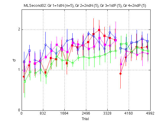
Average REFERENCE DIRECTION out to make two supergroups: First and Second
Based on visual inspection of the above plot, as well as knowledge of other data sets in our lab, the positive and negative directions of motion seem to yeild identical learning patterns. The red and magenta lines are right on top of each other. The blue and green lines seem equivalent up to multiplication by a constant factor. Thus, we are going to combine Group 1+3 into a (super)Group 1 and Groups 2+4 into sGroup 2.
1stN(1) + 1stP(3) --> First(1) ; 2ndN(2) + 2ndP(4) --> Second(2)
l_gr4 = {'Gr 1=1stN','Gr 2=2ndN','Gr 3=1stP','Gr 4=2ndP'} ; % old legend
l = {'Gr 1=First','Gr 2=Second'} ; % new legend
Ss2{1} = [Ss4{1} , Ss4{3}] ;
Ss2{2} = [Ss4{2} , Ss4{4}] ;
assert(isempty(intersect(Ss2{1},Ss2{2}))) ; % Sanity check
N_sbj_gr2 = N_sbj_gr4(1:2) + N_sbj_gr4(3:4) ;
madpr2 = (madpr2_gr4(:,1:2)+madpr2_gr4(:,3:4))./2 ;
semadpr2 = (semadpr2_gr4(:,1:2)+semadpr2_gr4(:,3:4))./2 ;
medpr2 = (medpr2_gr4(:,1:2)+medpr2_gr4(:,3:4))./2 ;
semedpr2 = (semedpr2_gr4(:,1:2)+semedpr2_gr4(:,3:4))./2 ;
mhdpr2 = (mhdpr2_gr4(:,1:2)+mhdpr2_gr4(:,3:4))./2 ;
semhdpr2 = (semhdpr2_gr4(:,1:2)+semhdpr2_gr4(:,3:4))./2 ;
% within-sbj confidence intervals
CI_madpr2 = z_crit.*(semadpr2./repmat(sqrt(N_sbj_gr2),N_blocks2,1)) ;
CI_medpr2 = z_crit.*(semedpr2./repmat(sqrt(N_sbj_gr2),N_blocks2,1)) ;
CI_mhdpr2 = z_crit.*(semhdpr2./repmat(sqrt(N_sbj_gr2),N_blocks2,1)) ;
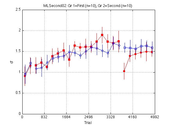
Plot adprime2 for the two (super)groups
clr = 'rb' ;      % Red=1stN, Blue=2ndN, Magenta=1stP, Green=2ndP
JTR2 = [-.5 .5].*(trials_block/8) ;     % jitter for visibility
train_first_p = [true false] ;        % controls MarkerFaceColor
sym1 = 'os' ;    % transfer order of motion: square=1st, circle=2nd
sym2 = 'so' ;    % training order of motion: square=1st, circle=2nd
M = 2.5 ;  % max d'

clf
d = madpr2 ;   % plot all_dprime2 averaged into 2 groups
CI = CI_madpr2 ;
for k = 1:2
    hold on ;  % must be inside the loop
    t = gT + JTR2(k) ;
    C = clr(k) ;      % color for this group. Always remains consistent
    s1 = sym1(k) ;    % transfer symbol for this group
    s2 = sym2(k) ;    % training symbol for this group
    h = plot(...
        t(i1) ,d(i1,k) ,[C s1 '-']   ... % 1: pre-test
       ,t(i2) ,d(i2,k) ,[C s2 '-']   ... % 2: train
       ,t(i3) ,d(i3,k) ,[C s1 '-']   ... % 3: post-test
       ) ;
    % Filled symbols demarkate groups training on first-order stimuli
    if (train_first_p(k))
        set(h,'MarkerFaceColor',C) ;
    %else  leave symbols open
    end
    % Error bars w/in Ss.  (This call contains an implicit 'hold off')
    errorbar1(t,d(:,k),CI(:,k),[C 'n']) ;   % no whiskers
end
hold off ; box on ;
clear d CI h

axis([0 N_trials 0 M]) ; grid on ;
set(gca,'xtick',xtick,'ytick',(0:.5:M)) ;
xlabel('Trial') ; ylabel('d''') ;
title(sprintf('MLSecond02: %s (n=%d), %s (n=%d) '  ...
     ,l{1},N_sbj_gr2(1),l{2},N_sbj_gr2(2) ));
Plot easy and hard d' separately
clr = 'rbrb' ;      % Red=1st, Blue=2nd; Repeat for Easy and Hard
train_first_p = [true false true false] ;    % controls MarkerFaceColor
sym1 = 'osos' ;    % transfer: square=1st, circle=2nd; Repeat Ez & Hd
sym2 = 'soso' ;    % training: square=1st, circle=2nd; Repeat Ez & Hd

clf
d = [medpr2 mhdpr2] ;   % [easy_dprime2 hard_dprime2], N_blocks2-by-4
CI = [CI_medpr2 CI_mhdpr2] ;
for k = 1:4
    hold on ;  % must be inside the loop
    t = gT + JTR4(k) ;
    C = clr(k) ;      % color for this group. Always remains consistent
    s1 = sym1(k) ;    % transfer symbol for this group
    s2 = sym2(k) ;    % training symbol for this group
    h = plot(...
        t(i1)  ,d(i1,k) ,[C s1 '-']   ... % 1: pre-test
       ,t(i2)  ,d(i2,k) ,[C s2 '-']   ... % 2: train
       ,t(i3)  ,d(i3,k) ,[C s1 '-']   ... % 3: post-test
       ) ;
    % Filled symbols demarkate groups training on first-order stimuli
    if (train_first_p(k))
        set(h,'MarkerFaceColor',C) ;
    %else  leave symbols open
    end

    % Error bars w/in Ss.  (This call contains an implicit 'hold off')
    errorbar1(t,d(:,k),CI(:,k),[C 'n']) ;   % no whiskers
end
hold off ; box on ;
clear d CI h

axis([0 N_trials 0 M]) ; grid on ;
set(gca,'xtick',xtick,'ytick',(0:.5:M)) ;
xlabel('Trial') ; ylabel('d''') ;
title(sprintf('MLSecond02: %s (n=%d), %s (n=%d). Easy and difficult delta ' ...
     ,l{1},N_sbj_gr2(1),l{2},N_sbj_gr2(2) ));

Prepare to run MLZ02_lsqcurvefit: Saturated model
main_ydata = [medpr2 mhdpr2] ;
main_ydata_CI = [CI_medpr2 CI_mhdpr2] ;  % within Ss

% Group interpretation -- index the columns of main_ydata and rows of params
G.EzGr1 = 1 ;
G.EzGr2 = 2 ;
G.HdGr1 = 3 ;
G.HdGr2 = 4 ;
G.descr = {'EzGr1', 'EzGr2', 'HdGr1', 'HdGr2'} ;

% Problem struct for fitting the saturated model via MLZ02_lsqcurvefit.
% Subsequent reduced models will be built on this basis
saturated_problem = MLZ02_lsqcurvefit ;   % default struct
saturated_problem.comment = 'Fully saturated model: 4*8 params total' ;
saturated_problem.group_idx = G ;

saturated_problem.xdata = xdata ;        % generated by MLZ02_piecemeal_curve
saturated_problem.ydata = main_ydata ;   % [N_blocks2 x 4]

% Parameter interpetation. See MLZ02_piecemeal_curve for details.
I = xdata.params_idx ;
% I.Y1 = 1 ;      % test1_Ybeg
% I.Y2 = 2 ;      % test1_Yend
% I.Y3 = 3 ;      % train_Ybeg
% I.Y18 = 4 ;     % train_Yend
% I.Y19 = 5 ;     % test2_Ybeg
% I.Y24 = 6 ;     % test2_Yend
% I.Tau = 7 ;     % train_tau
% I.Tau2 = 8 ;    % test2_tau

% Lower and Upper bounds for the parameter search
lb1 = NaN(1,8) ;
lb1([I.Y1 I.Y2 I.Y3 I.Y18 I.Y19 I.Y24]) = 0 ;  % min d'
lb1([I.Tau I.Tau2]) = 10 ;                     % min time constant (in trials)

ub1 = NaN(1,8) ;
ub1([I.Y1 I.Y2 I.Y3 I.Y18 I.Y19 I.Y24]) = 4 ;  % max d'
ub1([I.Tau I.Tau2]) = 10000 ;                  % max time constant (in trials)

saturated_problem.lb_x = repmat(lb1,4,1) ;
saturated_problem.ub_x = repmat(ub1,4,1) ;

% Start the search with values taken from main ydata
main_params0 = NaN(4,8) ;      % 4 groups x 8 parameters each
main_params0(:,I.Y1)  = main_ydata(1,:)' ;
main_params0(:,I.Y2)  = main_ydata(2,:)' ;
main_params0(:,I.Y3)  = main_ydata(3,:)' ;
main_params0(:,I.Y18) = mean(main_ydata(16:18,:))' ;
main_params0(:,I.Y19) = main_ydata(19,:)' ;
main_params0(:,I.Y24) = mean(main_ydata(23:24,:))' ;
main_params0(:,I.Tau) = 1600 ;
main_params0(:,I.Tau2)= 150 ;
saturated_problem.params0 = main_params0 ;
saturated_problem.x0 = saturated_problem.param2vect(main_params0)

% Optimization options. See optimset('lsqnonlin') for details
%saturated_problem.options.Display = 'iter' ;  % verbose optimization

% R-squared utility
%subsref1 = @(vect,idx) (vect(idx)) ;   % now in utils/general
Rsq = @(x,y) (subsref1(corrcoef(x(:),y(:)),2)^2) ;
saturated_problem =

         comment: 'Fully saturated model: 4*8 params total'
           xdata: [1x1 struct]
           ydata: [24x4 double]
      vect2param: @(x)(x)
      param2vect: @(p)(p)
    vector_names: {'Y1'  'Y2'  'Y3'  'Y18'  'Y19'  'Y24'  'tau'  'tau2'}
              x0: [4x8 double]
         params0: [4x8 double]
            lb_x: [4x8 double]
            ub_x: [4x8 double]
         options: [1x1 struct]
       group_idx: [1x1 struct]
Fit the saturated model
saturated_fit = MLZ02_lsqcurvefit(saturated_problem)   % <-- Sic!

fprintf('\nGroup:    Y1    Y2      Y3   Y18     Y19   Y24     Tau  Tau2 \n') ;
for k = 1:4
    p = saturated_fit.opt_params(k,:) ;
    fprintf('%s: %5.2f %5.2f   %5.2f %5.2f   %5.2f %5.2f   %5d %5d \n' ...
           ,G.descr{k} ...
           ,p(I.Y1),p(I.Y2), p(I.Y3),p(I.Y18), p(I.Y19),p(I.Y24)   ...
           ,round(p(I.Tau)), round(p(I.Tau2)) ) ;
end
saturated_fit =
comment: 'Fully saturated model: 4*8 params total'
opt_x: [4x8 double]
opt_params: [4x8 double]
yhat: [24x4 double]
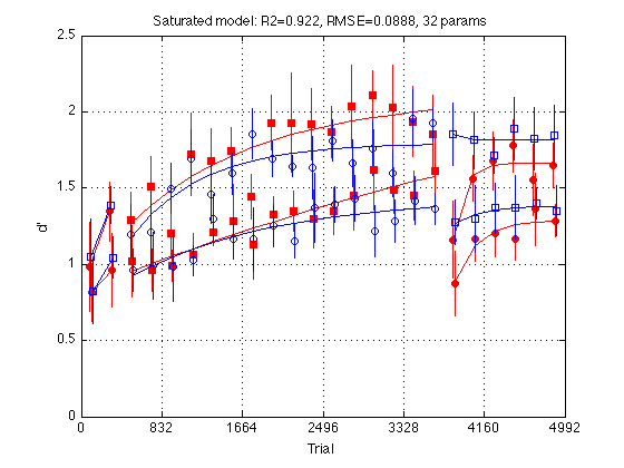
RMSE: 0.0888
R2: 0.9218
exitflag: 3
output: [1x1 struct]
Group: Y1 Y2 Y3 Y18 Y19 Y24 Tau Tau2
EzGr1: 0.98 1.35 1.27 2.01 1.16 1.67 1369 118
EzGr2: 1.05 1.39 1.18 1.79 1.86 1.82 756 10
HdGr1: 0.81 0.96 0.96 1.58 0.89 1.29 7479 240
HdGr2: 0.82 1.04 0.93 1.38 1.27 1.38 1539 332
Plot the fit of the saturated model
clf
d = saturated_problem.ydata ;
CI = [CI_medpr2 CI_mhdpr2] ;
f = saturated_fit.yhat ;
for k = 1:4
    hold on ;  % must be inside the loop
    t = gT + JTR4(k) ;
    C = clr(k) ;      % color for this group. Always remains consistent
    s1 = sym1(k) ;    % transfer symbol for this group
    s2 = sym2(k) ;    % training symbol for this group
    h = plot(...
        t(i1)  ,d(i1,k) ,[C s1]   ... % 1: pre-test data
       ,t(i1)  ,f(i1,k) ,[C '-']  ... % 1: pre-test fit
       ,t(i2)  ,d(i2,k) ,[C s2]   ... % 2: train data
       ,t(i2)  ,f(i2,k) ,[C '-']  ... % 2: train fit
       ,t(i3)  ,d(i3,k) ,[C s1]   ... % 3: post-test data
       ,t(i3)  ,f(i3,k) ,[C '-']  ... % 3: post-test fit
       ) ;
    % Filled symbols demarkate groups training on first-order stimuli
    if (train_first_p(k))
        set(h,'MarkerFaceColor',C) ;
    %else  leave symbols open
    end
    % Error bars w/in Ss.  (This call contains an implicit 'hold off')
    errorbar1(t,d(:,k),CI(:,k),[C 'n']) ;   % no whiskers
end
hold off ; box on ;
clear d CI h f

axis([0 N_trials 0 M]) ; grid on ;
set(gca,'xtick',xtick,'ytick',(0:.5:M)) ;
xlabel('Trial') ; ylabel('d''') ;
title(sprintf('Saturated model: R2=%.3f, RMSE=%.4f, 32 params ' ...
     ,saturated_fit.R2 ,saturated_fit.RMSE ));
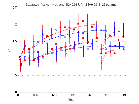
Saturated model with common time constants
The time constants tau are poorly constrained by the data. It should be easy to fit all four groups with the same Tau and Tau2. The Yxx params are still separate for each group. Thus this model has 26=4*6+2 params.
% Representation scheme: X is a 1x26 vector. X(25)=Tau, X(26)=Tau2.
saturY_cmnTau_vector_names = { ...
    'EzGr1Y1' 'EzGr1Y2' 'EzGr1Y3' 'EzGr1Y18' 'EzGr1Y19' 'EzGr1Y24' ...
    'EzGr2Y1' 'EzGr2Y2' 'EzGr2Y3' 'EzGr2Y18' 'EzGr2Y19' 'EzGr2Y24' ...
    'HdGr1Y1' 'HdGr1Y2' 'HdGr1Y3' 'HdGr1Y18' 'HdGr1Y19' 'HdGr1Y24' ...
    'HdGr2Y1' 'HdGr2Y2' 'HdGr2Y3' 'HdGr2Y18' 'HdGr2Y19' 'HdGr2Y24' ...
    'tau' 'tau2' } ;

saturY_cmnTau_vect2param = @(x) ...
    ([x( 1: 6) x(25) x(26) ...  % Gr 1: EzGr1
     ;x( 7:12) x(25) x(26) ...  % Gr 2: EzGr2
     ;x(13:18) x(25) x(26) ...  % Gr 3: HdGr1
     ;x(19:24) x(25) x(26) ]) ; % Gr 4: HdGr2

saturY_cmnTau_param2vect = @(p) ...
    ([p(1,1:6) p(2,1:6) p(3,1:6) p(4,1:6) ...  % Group-specific Yxx
     ,p(1,7) p(1,8) ]) ;                       % Common Tau and Tau2

% Construct a new problem structure based on saturated_problem:
saturY_cmnTau_problem = saturated_problem ;
saturY_cmnTau_problem.comment = 'Saturated Yxx, common Tau''s' ;
saturY_cmnTau_problem.vect2param = saturY_cmnTau_vect2param ;
saturY_cmnTau_problem.param2vect = saturY_cmnTau_param2vect ;
saturY_cmnTau_problem.vector_names = saturY_cmnTau_vector_names ;

% Start the new search from saturated_fit.opt_params:
x = saturY_cmnTau_param2vect(saturated_fit.opt_params) ;
x(25) = 1600 ;    % guess for the common Tau
x(26) =  150 ;    % guess for the common Tau2
saturY_cmnTau_problem.x0 = x ;

p = saturY_cmnTau_vect2param(x) ;
saturY_cmnTau_problem.params0 = p ;
assert(all(x==saturY_cmnTau_param2vect(p))) ;  % Sanity check

% Inherit the bounds from saturated_problem:
p = saturated_problem.vect2param(saturated_problem.lb_x) ; % canonicalize
x = saturY_cmnTau_param2vect(p) ;
assert(all(all(p==saturY_cmnTau_vect2param(x)))) ;  % Sanity check
saturY_cmnTau_problem.lb_x = x ;

p = saturated_problem.vect2param(saturated_problem.ub_x) ; % canonicalize
x = saturY_cmnTau_param2vect(p) ;
assert(all(all(p==saturY_cmnTau_vect2param(x)))) ;  % Sanity check
saturY_cmnTau_problem.ub_x = x           %#ok<NOPTS>
saturY_cmnTau_problem =

         comment: 'Saturated Yxx, common Tau's'
           xdata: [1x1 struct]
           ydata: [24x4 double]
      vect2param: @(x)([x(1:6),x(25),x(26);x(7:12),x(25),x(26);x(13:18),x(25),x(26);x(19:24),x(25),x(26)])
      param2vect: @(p)([p(1,1:6),p(2,1:6),p(3,1:6),p(4,1:6),p(1,7),p(1,8)])
    vector_names: {1x26 cell}
              x0: [1x26 double]
         params0: [4x8 double]
            lb_x: [0 0 0 0 0 0 0 0 0 0 0 0 0 0 0 0 0 0 0 0 0 0 0 0 10 10]
            ub_x: [4 4 4 4 4 4 4 4 4 4 4 4 4 4 4 4 4 4 4 4 4 4 4 4 10000 10000]
         options: [1x1 struct]
       group_idx: [1x1 struct]
Fit the saturated model with common time constants
saturY_cmnTau_fit = MLZ02_lsqcurvefit(saturY_cmnTau_problem)   %#ok<NOPTS>

fprintf('\nGroup:    Y1    Y2      Y3   Y18     Y19   Y24     Tau  Tau2 \n') ;
for k = 1:4
    p = saturY_cmnTau_fit.opt_params(k,:) ;
    fprintf('%s: %5.2f %5.2f   %5.2f %5.2f   %5.2f %5.2f   %5d %5d \n' ...
           ,G.descr{k} ...
           ,p(I.Y1),p(I.Y2), p(I.Y3),p(I.Y18), p(I.Y19),p(I.Y24)   ...
           ,round(p(I.Tau)), round(p(I.Tau2)) ) ;
end
saturY_cmnTau_fit =

       comment: 'Saturated Yxx, common Tau's'
         opt_x: [1x26 double]
    opt_params: [4x8 double]
          yhat: [24x4 double]
          RMSE: 0.0918
            R2: 0.9165
      exitflag: 3
        output: [1x1 struct]


Group:    Y1    Y2      Y3   Y18     Y19   Y24     Tau  Tau2
EzGr1:  0.98  1.35    1.29  2.02    1.16  1.67    1598   141
EzGr2:  1.05  1.39    1.27  1.84    1.85  1.82    1598   141
HdGr1:  0.81  0.96    0.89  1.51    0.87  1.26    1598   141
HdGr2:  0.82  1.04    0.93  1.38    1.27  1.37    1598   141
Significance test for nested multiple regression models
F-test of nested multiple regression models (see Equation on p. 542 in Howell, D. C. (1992), "Statistical Methods for Psychology", 3rd Ed.)
                (N-f-1)*(R2f-R2r)
F(f-r,N-f-1) = -------------------
                  (f-r)*(1-R2f)
N is the number of observations, R2F and R2R are the squared multiple correlations for the full and reduced models, respectively. DF_F and DF_R are the corresponding degrees of freedom. When not specified, the reduced model defaults to zero and thus the function calculates a test of whether R2F is significantly greater than zero. When two models are specified, the test is whether the increment of R2 is significant. See utils/R2signif.m for details.
Strictly speaking, this test is mathematically impeccable only for linear regression, but we're going to use it regardless. With the exception of the two tau's, our model is (quasi)linear in the parameters.
% Test the transition saturated_problem --> saturY_cmnTau_problem:
N_data_points = numel(main_ydata) ;   % 96 independent observations
Mf = saturated_fit ;       % full model
Mr = saturY_cmnTau_fit ;   % reduced model
df_f = numel(Mf.opt_x) ;   % degrees of freedom (# params) full model
df_r = numel(Mr.opt_x) ;   % degrees of freedom (# params) reduced model
[F,p] = R2signif(N_data_points,Mf.R2,df_f,Mr.R2,df_r) ;
fprintf('Full:         R2=%.4f, df=%2d  (%s)\n',Mf.R2,df_f,Mf.comment) ;
fprintf('Reduced:      R2=%.4f, df=%2d  (%s)\n',Mr.R2,df_r,Mr.comment) ;
fprintf('Significance: F(%d,%d)=%.4f, p=%.8f\n' ...
       , df_f-df_r, N_data_points-df_f-1, F, p) ;

% Conclusion: The drop in R2 (.9218 --> .9165) is not statistically
% significant and more than justifies the elimination of 6 free parameters.
Full:         R2=0.9218, df=32  (Fully saturated model: 4*8 params total)
Reduced:      R2=0.9165, df=26  (Saturated Yxx, common Tau's)
Significance: F(6,63)=0.7080, p=0.64433546
Plot the fit of the saturated model with common time constants
clf
d = saturY_cmnTau_problem.ydata ;
CI = [CI_medpr2 CI_mhdpr2] ;
f = saturY_cmnTau_fit.yhat ;
for k = 1:4
    hold on ;  % must be inside the loop
    t = gT + JTR4(k) ;
    C = clr(k) ;      % color for this group. Always remains consistent
    s1 = sym1(k) ;    % transfer symbol for this group
    s2 = sym2(k) ;    % training symbol for this group
    h = plot(...
        t(i1)  ,d(i1,k) ,[C s1]   ... % 1: pre-test data
       ,t(i1)  ,f(i1,k) ,[C '-']  ... % 1: pre-test fit
       ,t(i2)  ,d(i2,k) ,[C s2]   ... % 2: train data
       ,t(i2)  ,f(i2,k) ,[C '-']  ... % 2: train fit
       ,t(i3)  ,d(i3,k) ,[C s1]   ... % 3: post-test data
       ,t(i3)  ,f(i3,k) ,[C '-']  ... % 3: post-test fit
       ) ;
    % Filled symbols demarkate groups training on first-order stimuli
    if (train_first_p(k))
        set(h,'MarkerFaceColor',C) ;
    %else  leave symbols open
    end
    % Error bars w/in Ss.  (This call contains an implicit 'hold off')
    errorbar1(t,d(:,k),CI(:,k),[C 'n']) ;   % no whiskers
end
hold off ; box on ;
clear d CI h f

axis([0 N_trials 0 M]) ; grid on ;
set(gca,'xtick',xtick,'ytick',(0:.5:M)) ;
xlabel('Trial') ; ylabel('d''') ;
title(sprintf('Saturated Yxx, common taus: R2=%.3f, RMSE=%.4f, 26 params ' ...
     ,saturY_cmnTau_fit.R2 ,saturY_cmnTau_fit.RMSE ));
Proportionality between Easy and Hard d'
For both groups, the Yxx parameters for the Easy delta are proportional to that for the Hard delta. The ratio is ~1.345 and is the same for both groups:
p = saturY_cmnTau_fit.opt_params ;
p = p(1:2,:)./p(3:4,:)    %#ok<NOPTS>
f = geomean(p(:,1:6),2)   %#ok<NOPTS>
geomean(f)
p =

    1.2087    1.3982    1.4476    1.3426    1.3375    1.3296    1.0000    1.0000
    1.2810    1.3292    1.3654    1.3368    1.4578    1.3295    1.0000    1.0000


f =

    1.3420
    1.3489


ans =

    1.3454
Independent-group model with Easy/Hard proportionality
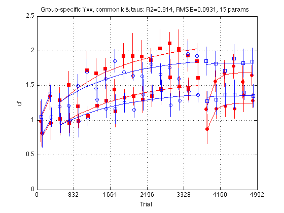
The Yxx for the Easy delta in each group is proportional to the Yxx for the Hard delta in the same group. The two groups have separate hard Yxx params. The coefficient of proportionality k is the same for both groups. The time constants Tau and Tau2 are also the same. Total number of params: 6+6+2+1=15
% Representation scheme: X is a 1x15 vector. X(13)=k, X(14)=Tau, X(15)=Tau2.
indepGr_cmnKTau_vector_names = { ...
    'HdGr1Y1' 'HdGr1Y2' 'HdGr1Y3' 'HdGr1Y18' 'HdGr1Y19' 'HdGr1Y24' ...
    'HdGr2Y1' 'HdGr2Y2' 'HdGr2Y3' 'HdGr2Y18' 'HdGr2Y19' 'HdGr2Y24' ...
    'k'       'tau'     'tau2' } ;
indepGr_K_idx = 13 ;

indepGr_cmnKTau_vect2param = @(x) ...
    ([x(13).*x(1: 6) x(14) x(15) ...  % Gr 1: EzGr1
     ;x(13).*x(7:12) x(14) x(15) ...  % Gr 2: EzGr2
     ;       x(1: 6) x(14) x(15) ...  % Gr 3: HdGr1
     ;       x(7:12) x(14) x(15) ]) ; % Gr 4: HdGr2

indepGr_cmnKTau_param2vect = @(p) ...
    ([p(3,1:6) p(4,1:6)           ...        % HdGr1_Yxx  HdGr2_Yxx
     ,geomean([geomean(p(1,1:6)./p(3,1:6))   ... % geomean([Gr1_k,Gr2_k])
              ,geomean(p(2,1:6)./p(4,1:6))]) ...
     ,p(1,7) p(1,8) ]) ;                     % Common Tau and Tau2

% Construct a new problem structure based on saturated_problem:
indepGr_cmnKTau_problem = saturated_problem ;
indepGr_cmnKTau_problem.comment = 'Group-specific Yxx, common k & Tau''s' ;
indepGr_cmnKTau_problem.vect2param = indepGr_cmnKTau_vect2param ;
indepGr_cmnKTau_problem.param2vect = indepGr_cmnKTau_param2vect ;
indepGr_cmnKTau_problem.vector_names = indepGr_cmnKTau_vector_names ;

% Start the new search from saturY_cmnTau_fit.opt_params:
x = indepGr_cmnKTau_param2vect(saturY_cmnTau_fit.opt_params) ;
indepGr_cmnKTau_problem.x0 = x ;

p = indepGr_cmnKTau_vect2param(x) ;
indepGr_cmnKTau_problem.params0 = p ;
assert(all(x==indepGr_cmnKTau_param2vect(p))) ;  % Sanity check

% Inherit the bounds from saturated_problem:
p = saturated_problem.vect2param(saturated_problem.lb_x) ;  % canonicalize
x = indepGr_cmnKTau_param2vect(p) ;
x(indepGr_K_idx) = 1.0 ;     % lower bound on k. This mandates that EzYxx>=HdYxxx
assert(all(all(p==indepGr_cmnKTau_vect2param(x)))) ;  % Sanity check
indepGr_cmnKTau_problem.lb_x = x ;

p = saturated_problem.vect2param(saturated_problem.ub_x) ;  % canonicalize
x = indepGr_cmnKTau_param2vect(p) ;
assert(all(all(p==indepGr_cmnKTau_vect2param(x)))) ;  % Sanity check
x(indepGr_K_idx) = 2.0 ;     % upper bound on k
indepGr_cmnKTau_problem.ub_x = x      %#ok<NOPTS>

% Optimization options. See optimset('lsqnonlin') for details
%indepGr_cmnKTau_problem.options.Display = 'iter' ;  % verbose optimization
indepGr_cmnKTau_problem =

         comment: 'Group-specific Yxx, common k & Tau's'
           xdata: [1x1 struct]
           ydata: [24x4 double]
      vect2param: [1x1 function_handle]
      param2vect: [function_handle]
    vector_names: {1x15 cell}
              x0: [1x15 double]
         params0: [4x8 double]
            lb_x: [0 0 0 0 0 0 0 0 0 0 0 0 1 10 10]
            ub_x: [4 4 4 4 4 4 4 4 4 4 4 4 2 10000 10000]
         options: [1x1 struct]
       group_idx: [1x1 struct]
Fit the independent-group model with Easy/Hard proportionality
indepGr_cmnKTau_fit = MLZ02_lsqcurvefit(indepGr_cmnKTau_problem)   %#ok<NOPTS>

fprintf('\nGroup:    Y1    Y2      Y3   Y18     Y19   Y24     Tau  Tau2 \n') ;
for k = 1:4
    p = indepGr_cmnKTau_fit.opt_params(k,:) ;
    fprintf('%s: %5.2f %5.2f   %5.2f %5.2f   %5.2f %5.2f   %5d %5d \n' ...
           ,G.descr{k} ...
           ,p(I.Y1),p(I.Y2), p(I.Y3),p(I.Y18), p(I.Y19),p(I.Y24)   ...
           ,round(p(I.Tau)), round(p(I.Tau2)) ) ;
end
fprintf('EzYxx/HdYxx = k = %.4f \n\n',indepGr_cmnKTau_fit.opt_x(indepGr_K_idx)) ;

% Test the transition saturY_cmnTau_problem --> indepGr_cmnKTau_problem
Mf = saturY_cmnTau_fit ;   % full model
Mr = indepGr_cmnKTau_fit ; % reduced model
df_f = numel(Mf.opt_x) ;   % degrees of freedom (# params) full model
df_r = numel(Mr.opt_x) ;   % degrees of freedom (# params) reduced model
[F,p] = R2signif(N_data_points,Mf.R2,df_f,Mr.R2,df_r) ;
fprintf('Full:         R2=%.4f, df=%2d  (%s)\n',Mf.R2,df_f,Mf.comment) ;
fprintf('Reduced:      R2=%.4f, df=%2d  (%s)\n',Mr.R2,df_r,Mr.comment) ;
fprintf('Significance: F(%d,%d)=%.4f, p=%.8f\n' ...
       , df_f-df_r, N_data_points-df_f-1, F, p) ;

% Conclusion: The drop in R2 (.9165 --> .9140) is not statistically
% significant and more than justifies the elimination of 11 free params!
indepGr_cmnKTau_fit =

       comment: 'Group-specific Yxx, common k & Tau's'
         opt_x: [1x15 double]
    opt_params: [4x8 double]
          yhat: [24x4 double]
          RMSE: 0.0931
            R2: 0.9140
      exitflag: 3
        output: [1x1 struct]


Group:    Y1    Y2      Y3   Y18     Y19   Y24     Tau  Tau2
EzGr1:  1.02  1.33    1.26  2.03    1.17  1.68    1561   140
EzGr2:  1.07  1.39    1.26  1.85    1.80  1.83    1561   140
HdGr1:  0.76  0.98    0.93  1.50    0.87  1.25    1561   140
HdGr2:  0.79  1.03    0.93  1.37    1.33  1.35    1561   140
EzYxx/HdYxx = k = 1.3507

Full:         R2=0.9165, df=26  (Saturated Yxx, common Tau's)
Reduced:      R2=0.9140, df=15  (Group-specific Yxx, common k & Tau's)
Significance: F(11,69)=0.1891, p=0.99775495
Plot the fit of the independent-group model with Easy/Hard proportionality
clf
d = indepGr_cmnKTau_problem.ydata ;
CI = [CI_medpr2 CI_mhdpr2] ;
f = indepGr_cmnKTau_fit.yhat ;
for k = 1:4
    hold on ;  % must be inside the loop
    t = gT + JTR4(k) ;
    C = clr(k) ;      % color for this group. Always remains consistent
    s1 = sym1(k) ;    % transfer symbol for this group
    s2 = sym2(k) ;    % training symbol for this group
    h = plot(...
        t(i1)  ,d(i1,k) ,[C s1]   ... % 1: pre-test data
       ,t(i1)  ,f(i1,k) ,[C '-']  ... % 1: pre-test fit
       ,t(i2)  ,d(i2,k) ,[C s2]   ... % 2: train data
       ,t(i2)  ,f(i2,k) ,[C '-']  ... % 2: train fit
       ,t(i3)  ,d(i3,k) ,[C s1]   ... % 3: post-test data
       ,t(i3)  ,f(i3,k) ,[C '-']  ... % 3: post-test fit
       ) ;
    % Filled symbols demarkate groups training on first-order stimuli
    if (train_first_p(k))
        set(h,'MarkerFaceColor',C) ;
    %else  leave symbols open
    end
    % Error bars w/in Ss.  (This call contains an implicit 'hold off')
    errorbar1(t,d(:,k),CI(:,k),[C 'n']) ;   % no whiskers
end
hold off ; box on ;
clear d CI h f

axis([0 N_trials 0 M]) ; grid on ;
set(gca,'xtick',xtick,'ytick',(0:.5:M)) ;
xlabel('Trial') ; ylabel('d''') ;
title(sprintf('Group-specific Yxx, common k & taus: R2=%.3f, RMSE=%.4f, 15 params ' ...
     ,indepGr_cmnKTau_fit.R2 ,indepGr_cmnKTau_fit.RMSE ));
Twelve-parameter model: Common Y1, Y2, Y3
Our pilot experiment has been remarkably successful in equalizing the initial performance level in the two groups. Constrain the Y1, Y2, and Y3 parameters to be common in the two groups. K, tau, tau2 remain shared. Total number of params: 3+2*3+1+2=12
% Representation scheme: X is a 1x12 vector:
% x(1:3) stores [Y1 Y2 Y3] for both Hard groups
% x(4:6) stores [Y18 Y19 Y24] for HdGr1
% x(7:9) stores [Y18 Y19 Y24] for HdGr2
% x(10) stores k = EzYxx/HdYxx for both groups
% x(11) and x(12) store Tau and Tau2 for both groups
param12_vector_names = { ...
    'HdY1'     'HdY2'     'HdY3'     ...   % 1:3
    'HdGr1Y18' 'HdGr1Y19' 'HdGr1Y24' ...   % 4:6
    'HdGr2Y18' 'HdGr2Y19' 'HdGr2Y24' ...   % 7:9
    'k'        'tau'      'tau2'     } ;   %10:12

param12_vect2param = @(x) ...
    ([ x(10).*x(1:3) ...  % EzGr1: [Y1  Y2  Y3 ]
      ,x(10).*x(4:6) ...  % EzGr1: [Y18 Y19 Y24]
      ,x(11), x(12)  ...  % EzGr1: [Tau Tau2]
     ; x(10).*x(1:3) ...  % EzGr2: [Y1  Y2  Y3 ]
      ,x(10).*x(7:9) ...  % EzGr2: [Y18 Y19 Y24]
      ,x(11), x(12)  ...  % EzGr2: [Tau Tau2]
     ;        x(1:3) ...  % HdGr1: [Y1  Y2  Y3 ]
      ,       x(4:6) ...  % HdGr1: [Y18 Y19 Y24]
      ,x(11), x(12)  ...  % HdGr2: [Tau Tau2]
     ;        x(1:3) ...  % HdGr2: [Y1  Y2  Y3 ]
      ,       x(7:9) ...  % HdGr2: [Y18 Y19 Y24]
      ,x(11), x(12)  ]);  % HdGr2: [Tau Tau2]

param12_param2vect = @(p) ...
    ([p(3,1:3) ...    % [Y1  Y2  Y3] for both Hard groups
     ,p(3,4:6) ...    % [Y18 Y19 Y24] for HdGr1
     ,p(4,4:6) ...    % [Y18 Y19 Y24] for HdGr2
     ,geomean([geomean(p(1,1:6)./p(3,1:6))   ... % geomean([Gr1_k,Gr2_k])
              ,geomean(p(2,1:6)./p(4,1:6))]) ...
     ,p(1,7) p(1,8) ]) ;                         % Common Tau and Tau2

% Construct a new problem structure based on saturated_problem:
param12_problem = saturated_problem ;
param12_problem.comment = 'Specific Y18,Y19,Y24. Common Y1,Y2,Y3, k, Tau,Tau2' ;
param12_problem.vect2param = param12_vect2param ;
param12_problem.param2vect = param12_param2vect ;
param12_problem.vector_names = param12_vector_names ;

% Start the new search from saturY_cmnTau_fit.opt_params:
x = param12_param2vect(saturY_cmnTau_fit.opt_params) ;
param12_problem.x0 = x ;

p = param12_vect2param(x) ;
param12_problem.params0 = p ;
assert(all(x==param12_param2vect(p))) ;  % Sanity check

% Inherit the bounds from saturated_problem:
p = saturated_problem.vect2param(saturated_problem.lb_x) ;  % canonicalize
x = param12_param2vect(p) ;
x(10) = 1.0 ;     % lower bound on k. This mandates that EzYxx>=HdYxxx
assert(max(max(abs(p-param12_vect2param(x))))<1e-6) ; % Sanity check
param12_problem.lb_x = x ;

p = saturated_problem.vect2param(saturated_problem.ub_x) ;  % canonicalize
x = param12_param2vect(p) ;
assert(max(max(abs(p-param12_vect2param(x))))<1e-6) ; % Sanity check
x(10) = 2.0 ;     % upper bound on k
param12_problem.ub_x = x      %#ok<NOPTS>

% Optimization options. See optimset('lsqnonlin') for details
%param12_problem.options.Display = 'iter' ;  % verbose optimization
param12_problem =

         comment: 'Specific Y18,Y19,Y24. Common Y1,Y2,Y3, k, Tau,Tau2'
           xdata: [1x1 struct]
           ydata: [24x4 double]
      vect2param: [function_handle]
      param2vect: [function_handle]
    vector_names: {1x12 cell}
              x0: [0.8134 0.9628 0.8900 1.5079 0.8710 1.2586 1.3773 1.2676 1.3664 1.3454 1.5977e+03 141.1831]
         params0: [4x8 double]
            lb_x: [0 0 0 0 0 0 0 0 0 1 10 10]
            ub_x: [4 4 4 4 4 4 4 4 4 2 10000 10000]
         options: [1x1 struct]
       group_idx: [1x1 struct]
Fit the twelve-parameter model
param12_fit = MLZ02_lsqcurvefit(param12_problem)   %#ok<NOPTS>

fprintf('\nGroup:    Y1    Y2      Y3   Y18     Y19   Y24     Tau  Tau2 \n') ;
for k = 1:4
    p = param12_fit.opt_params(k,:) ;
    fprintf('%s: %5.2f %5.2f   %5.2f %5.2f   %5.2f %5.2f   %5d %5d \n' ...
           ,G.descr{k} ...
           ,p(I.Y1),p(I.Y2), p(I.Y3),p(I.Y18), p(I.Y19),p(I.Y24)   ...
           ,round(p(I.Tau)), round(p(I.Tau2)) ) ;
end
fprintf('EzYxx/HdYxx = k = %.4f \n\n',param12_fit.opt_x(10)) ;

% Test the transition indepGr_cmnKTau_problem --> param12_problem
Mf = indepGr_cmnKTau_fit ; % full model
Mr = param12_fit ;         % reduced model
df_f = numel(Mf.opt_x) ;   % degrees of freedom (# params) full model
df_r = numel(Mr.opt_x) ;   % degrees of freedom (# params) reduced model
[F,p] = R2signif(N_data_points,Mf.R2,df_f,Mr.R2,df_r) ;
fprintf('Full:         R2=%.4f, df=%2d  (%s)\n',Mf.R2,df_f,Mf.comment) ;
fprintf('Reduced:      R2=%.4f, df=%2d  (%s)\n',Mr.R2,df_r,Mr.comment) ;
fprintf('Significance: F(%d,%d)=%.4f, p=%.8f\n' ...
       , df_f-df_r, N_data_points-df_f-1, F, p) ;

% Conclusion: The drop in R2 (.9140 --> .9135) is not statistically
% significant and more than justifies the elimination of 3 free params.
% The twelve-parameter model is a good candidate for being the final model.
% As of 2009-10-09, however, it is superseded by the "New Eleven-parameter
% model.
param12_fit =

       comment: 'Specific Y18,Y19,Y24. Common Y1,Y2,Y3, k, Tau,Tau2'
         opt_x: [0.7762 1.0085 0.9316 1.4999 0.8653 1.2456 1.3677 1.3326 1.3525 1.3508 1.5622e+03 140.1366]
    opt_params: [4x8 double]
          yhat: [24x4 double]
          RMSE: 0.0934
            R2: 0.9135
      exitflag: 3
        output: [1x1 struct]


Group:    Y1    Y2      Y3   Y18     Y19   Y24     Tau  Tau2
EzGr1:  1.05  1.36    1.26  2.03    1.17  1.68    1562   140
EzGr2:  1.05  1.36    1.26  1.85    1.80  1.83    1562   140
HdGr1:  0.78  1.01    0.93  1.50    0.87  1.25    1562   140
HdGr2:  0.78  1.01    0.93  1.37    1.33  1.35    1562   140
EzYxx/HdYxx = k = 1.3508

Full:         R2=0.9140, df=15  (Group-specific Yxx, common k & Tau's)
Reduced:      R2=0.9135, df=12  (Specific Y18,Y19,Y24. Common Y1,Y2,Y3, k, Tau,Tau2)
Significance: F(3,80)=0.1641, p=0.92027508
Plot the fit of the twelve-parameter model
clf
d = param12_problem.ydata ;
CI = [CI_medpr2 CI_mhdpr2] ;
f = param12_fit.yhat ;
train_easy_p = [true true false false] ; % Use to define easy and hard
circle_width_p = [false true false true] ; % Use to increase circle line width
for k = 1:4
    hold on ;  % must be inside the loop
    t = gT + JTR4(k) ;
    C = clr(k) ;      % color for this group. Always remains consistent
    s1 = sym1(k) ;    % transfer symbol for this group
    s2 = sym2(k) ;    % training symbol for this group
    h = plot(...
        t(i1)  ,d(i1,k) ,[C s1]   ... % 1: pre-test data
       ,t(i1)  ,f(i1,k) ,[C '-']  ... % 1: pre-test fit
       ,t(i2)  ,d(i2,k) ,[C s2]   ... % 2: train data
       ,t(i2)  ,f(i2,k) ,[C '-']  ... % 2: train fit
       ,t(i3)  ,d(i3,k) ,[C s1]   ... % 3: post-test data
       ,t(i3)  ,f(i3,k) ,[C '-']  ... % 3: post-test fit
       ) ;
    % Filled symbols demarkate groups training on first-order stimuli
    if (train_first_p(k))
        set(h,'MarkerFaceColor',C) ;
    %else  leave symbols open
    end
    % Large symbols demarkate easy delta
    if (train_easy_p(k))
        set(h,'Markersize',12) ;
    end
    % Increases line width for group 2 to make more visible
    if (circle_width_p(k))
        set(h,'LineWidth',1.1);
    end
    % Error bars w/in Ss.  (This call contains an implicit 'hold off')
    errorbar1(t,d(:,k),CI(:,k),[C 'n']) ;   % no whiskers
end
hold off ; box on ;
clear d CI h f

axis([0 N_trials 0 M]) ; grid on ;
set(gca,'xtick',xtick,'ytick',(0:.5:M)) ;
xlabel('Trial') ; ylabel('d''') ;
title(sprintf('MLSecond02: 12-param regression: R2=%.3f, RMSE=%.4f ' ...
     ,param12_fit.R2 ,param12_fit.RMSE ));

Eleven-parameter model: Common Y18
Intended to test the hypothesis that the learning during the training phase of the two groups are completely equivalent. That is, Y18 is also shared between the two groups, together with Y1, Y2, Y3, k, Tau, Tau2. Total number of params: 4+2*2+1+2=11
% Representation scheme: X is a 1x11 vector:
% x(1:4) stores [Y1 Y2 Y3 Y18] for both Hard groups
% x(5:6) stores [Y19 Y24] for HdGr1
% x(7:8) stores [Y19 Y24] for HdGr2
% x(9) stores k = EzYxx/HdYxx for both groups
% x(10) and x(11) store Tau and Tau2 for both groups
param11_vector_names = { ...
    'HdY1'     'HdY2'     'HdY3'   'HdY18'     ...   % 1:4
    'HdGr1Y19' 'HdGr1Y24'                      ...   % 5:6
    'HdGr2Y19' 'HdGr2Y24'                      ...   % 7:8
    'k'        'tau'      'tau2'     } ;             % 9:11

param11_vect2param = @(x) ...
    ([ x(9).*x(1:4) ...  % EzGr1: [Y1  Y2  Y3 Y18]
      ,x(9).*x(5:6) ...  % EzGr1: [Y19 Y24]
      ,x(10),x(11)  ...  % EzGr1: [Tau Tau2]
     ; x(9).*x(1:4) ...  % EzGr2: [Y1  Y2  Y3 Y18]
      ,x(9).*x(7:8) ...  % EzGr2: [Y19 Y24]
      ,x(10),x(11)  ...  % EzGr2: [Tau Tau2]
     ;       x(1:4) ...  % HdGr1: [Y1  Y2  Y3 Y18]
      ,      x(5:6) ...  % HdGr1: [Y19 Y24]
      ,x(10),x(11)  ...  % HdGr2: [Tau Tau2]
     ;       x(1:4) ...  % HdGr2: [Y1  Y2  Y3 Y18]
      ,      x(7:8) ...  % HdGr2: [Y19 Y24]
      ,x(10),x(11)  ]);  % HdGr2: [Tau Tau2]

param11_param2vect = @(p) ...
    ([p(3,1:4) ...    % [Y1  Y2 Y3 Y18] for both Hard groups
     ,p(3,5:6) ...    % [Y19 Y24] for HdGr1
     ,p(4,5:6) ...    % [Y19 Y24] for HdGr2
     ,geomean([geomean(p(1,1:6)./p(3,1:6))   ... % geomean([Gr1_k,Gr2_k])
              ,geomean(p(2,1:6)./p(4,1:6))]) ...
     ,p(1,7) p(1,8) ]) ;                         % Common Tau and Tau2

% Construct a new problem structure based on saturated_problem:
param11_problem = saturated_problem ;
param11_problem.comment = 'Specific Y19,Y24. Common Y1,Y2,Y3,Y18, k, Tau,Tau2' ;
param11_problem.vect2param = param11_vect2param ;
param11_problem.param2vect = param11_param2vect ;
param11_problem.vector_names = param11_vector_names ;

% Start the new search from param12_fit.opt_params:
x = param11_param2vect(param12_fit.opt_params) ;
param11_problem.x0 = x ;

p = param11_vect2param(x) ;
param11_problem.params0 = p ;
assert(all(x==param11_param2vect(p))) ;  % Sanity check

% Inherit the bounds from saturated_problem:
p = saturated_problem.vect2param(saturated_problem.lb_x) ;
x = param11_param2vect(p) ;
x(9) = 1.0 ;     % lower bound on k. This mandates that EzYxx>=HdYxxx
assert(max(max(abs(p-param11_vect2param(x))))<1e-6) ; % Sanity check
param11_problem.lb_x = x ;

p = saturated_problem.vect2param(saturated_problem.ub_x) ;
x = param11_param2vect(p) ;
assert(max(max(abs(p-param11_vect2param(x))))<1e-6) ; % Sanity check
x(9) = 2.0 ;     % upper bound on k
param11_problem.ub_x = x      %#ok<NOPTS>

% Optimization options. See optimset('lsqnonlin') for details
%param11_problem.options.Display = 'iter' ;  % verbose optimization
param11_problem =

         comment: 'Specific Y19,Y24. Common Y1,Y2,Y3,Y18, k, Tau,Tau2'
           xdata: [1x1 struct]
           ydata: [24x4 double]
      vect2param: [function_handle]
      param2vect: [function_handle]
    vector_names: {'HdY1'  'HdY2'  'HdY3'  'HdY18'  'HdGr1Y19'  'HdGr1Y24'  'HdGr2Y19'  'HdGr2Y24'  'k'  'tau'  'tau2'}
              x0: [0.7762 1.0085 0.9316 1.4999 0.8653 1.2456 1.3326 1.3525 1.3508 1.5622e+03 140.1366]
         params0: [4x8 double]
            lb_x: [0 0 0 0 0 0 0 0 1 10 10]
            ub_x: [4 4 4 4 4 4 4 4 2 10000 10000]
         options: [1x1 struct]
       group_idx: [1x1 struct]
Fit the eleven-parameter model
param11_fit = MLZ02_lsqcurvefit(param11_problem)   %#ok<NOPTS>

fprintf('\nGroup:    Y1    Y2      Y3   Y18     Y19   Y24     Tau  Tau2 \n') ;
for k = 1:4
    p = param11_fit.opt_params(k,:) ;
    fprintf('%s: %5.2f %5.2f   %5.2f %5.2f   %5.2f %5.2f   %5d %5d \n' ...
           ,G.descr{k} ...
           ,p(I.Y1),p(I.Y2), p(I.Y3),p(I.Y18), p(I.Y19),p(I.Y24)   ...
           ,round(p(I.Tau)), round(p(I.Tau2)) ) ;
end
fprintf('EzYxx/HdYxx = k = %.4f \n\n',param11_fit.opt_x(9)) ;

% Test the transition param12_problem --> param11_problem
Mf = param12_fit ;         % full model
Mr = param11_fit ;         % reduced model
df_f = numel(Mf.opt_x) ;   % degrees of freedom (# params) full model
df_r = numel(Mr.opt_x) ;   % degrees of freedom (# params) reduced model
[F,p] = R2signif(N_data_points,Mf.R2,df_f,Mr.R2,df_r) ;
fprintf('Full:         R2=%.4f, df=%2d  (%s)\n',Mf.R2,df_f,Mf.comment) ;
fprintf('Reduced:      R2=%.4f, df=%2d  (%s)\n',Mr.R2,df_r,Mr.comment) ;
fprintf('Significance: F(%d,%d)=%.4f, p=%.8f\n\n' ...
       , df_f-df_r, N_data_points-df_f-1, F, p) ;

% Conclusion: The drop in R2 (.9135 --> .8928) is highly statistically
% significant and cannot be offset by 1 additional degree of freedom.
% It is useful to repeat this analysis taking into account that only the
% training segment of the curve constrains the param12-->param11 nesting.
% This affects the total degrees of freedom and hence the p value.
df_f = 5 ;   % Y3, Y18_1, Y18_2, k, Tau
df_r = 4 ;   % Y3, Y18, k, Tau
N_training_points = 4*16 ;   % blocks 3-18 inclusive
[F,p] = R2signif(N_training_points,Mf.R2,df_f,Mr.R2,df_r) ;
fprintf('Full:         R2=%.4f, df=%2d  (%s)\n',Mf.R2,df_f,Mf.comment) ;
fprintf('Reduced:      R2=%.4f, df=%2d  (%s)\n',Mr.R2,df_r,Mr.comment) ;
fprintf('Significance: F(%d,%d)=%.4f, p=%.8f\n' ...
       , df_f-df_r, N_training_points-df_f-1, F, p) ;

% Conclusion: Still highly significant. The eleven-parameter model must be
% rejected in favor of the twelve-parameter model.

% *** Overall conclusion: ***
% The twelve parameter model offers a better description of the data.
% Note:  This does *not* mean that there is more learning in Group 1 than
% in Group 2 because the present analysis ignores the within-group
% variability across participants.  It is based on within-block variability
% of the group-averaged profiles.  These data are not independent when
% group comparisons are concerned and, therefore, cannot be used to
% establish significant *differences* between the groups. See the section
%"z-test whether there is more learning in Group 1 than in Group 2" for a
% bootstrap test that points that in fact the two groups are not
% significantly different.  [AP 2010-01-21]
param11_fit =

       comment: 'Specific Y19,Y24. Common Y1,Y2,Y3,Y18, k, Tau,Tau2'
         opt_x: [0.7762 1.0085 0.9285 1.4313 0.8654 1.2457 1.3327 1.3526 1.3506 1.4972e+03 140.1373]
    opt_params: [4x8 double]
          yhat: [24x4 double]
          RMSE: 0.1040
            R2: 0.8928
      exitflag: 3
        output: [1x1 struct]


Group:    Y1    Y2      Y3   Y18     Y19   Y24     Tau  Tau2
EzGr1:  1.05  1.36    1.25  1.93    1.17  1.68    1497   140
EzGr2:  1.05  1.36    1.25  1.93    1.80  1.83    1497   140
HdGr1:  0.78  1.01    0.93  1.43    0.87  1.25    1497   140
HdGr2:  0.78  1.01    0.93  1.43    1.33  1.35    1497   140
EzYxx/HdYxx = k = 1.3506

Full:         R2=0.9135, df=12  (Specific Y18,Y19,Y24. Common Y1,Y2,Y3, k, Tau,Tau2)
Reduced:      R2=0.8928, df=11  (Specific Y19,Y24. Common Y1,Y2,Y3,Y18, k, Tau,Tau2)
Significance: F(1,83)=19.8757, p=0.00002568

Full:         R2=0.9135, df= 5  (Specific Y18,Y19,Y24. Common Y1,Y2,Y3, k, Tau,Tau2)
Reduced:      R2=0.8928, df= 4  (Specific Y19,Y24. Common Y1,Y2,Y3,Y18, k, Tau,Tau2)
Significance: F(1,58)=13.8890, p=0.00044181
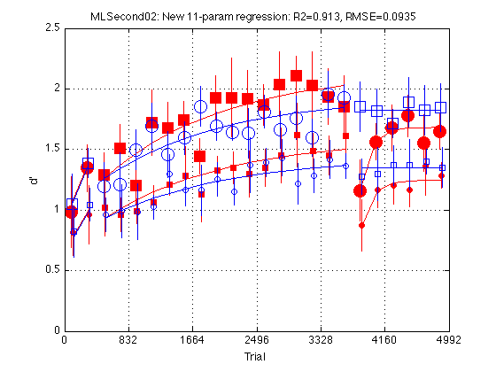
New Eleven-parameter model: HdGr2Y19==HdGr2Y24
Test a model in which the post-test beginning (Y19) and end (Y24) are common in Group 2 but are allowed to vary independently in Group 1.
Representation scheme: X is a 1x11 vector: x(1:3) stores [Y1 Y2 Y3] for both Hard groups x(4:6) stores [Y18 Y19 Y24] for HdGr1 x(7) stores [Y18] for HdGr2 x(8) stores [Y19==24] for HdGr2 x(9) stores k = EzYxx/HdYxx for both groups x(10) and x(11) store Tau and Tau2 for both groups
param11n_vector_names = { ...
    'HdY1'     'HdY2'     'HdY3'     ...   % 1:3
    'HdGr1Y18' 'HdGr1Y19' 'HdGr1Y24' ...   % 4:6
    'HdGr2Y18' 'HdGr2Y19'  ...             % 7:8
    'k'        'tau'      'tau2'     } ;   % 9:11
param11n_K_idx = 9 ;

param11n_vect2param = @(x) ...
    ([ x(9).*x(1:3) ...   % EzGr1: [Y1  Y2  Y3 ]
      ,x(9).*x(4:6) ...   % EzGr1: [Y18 Y19 Y24]
      ,x(10), x(11)  ...  % EzGr1: [Tau Tau2]
                    ...
     ; x(9).*x(1:3) ...   % EzGr2: [Y1  Y2  Y3 ]
      ,x(9).*x(7:8) ...   % EzGr2: [Y18 Y19]
      ,x(9).*x(8)   ...   % EzGr2: Y24==Y19
      ,x(10), x(11)  ...  % EzGr2: [Tau Tau2]
                     ...
     ;        x(1:3) ...  % HdGr1: [Y1  Y2  Y3 ]
      ,       x(4:6) ...  % HdGr1: [Y18 Y19 Y24]
      ,x(10), x(11)  ...  % HdGr1: [Tau Tau2]
                     ...
     ;        x(1:3) ...  % HdGr2: [Y1  Y2  Y3 ]
      ,       x(7:8) ...  % HdGr2: [Y18 Y19]
      ,       x(8)   ...  % HdGr2: Y24==Y19
      ,x(10), x(11)  ]);  % HdGr2: [Tau Tau2]

param11n_param2vect = @(p) ...
     ([p(3,1:3) ...    % [Y1  Y2  Y3] for both Hard groups
      ,p(3,4:6) ...    % [Y18 Y19 24] for HdGr1
      ,p(4,4:5) ...    % [Y18 Y19]    for HdGr2
      ,geomean([geomean(p(1,1:6)./p(3,1:6))   ... % geomean([Gr1_k,Gr2_k])
               ,geomean(p(2,1:6)./p(4,1:6))]) ...
      ,p(1,7) p(1,8) ]) ;                         % Common Tau and Tau2


% Construct a new problem structure based on saturated_problem:
param11n_problem = saturated_problem ;
param11n_problem.comment = 'Gr1: Y18,Y19,Y24; Gr2: Y18,Y19==Y24. Common Y1,Y2,Y3, k, Tau,Tau2' ;
param11n_problem.vect2param = param11n_vect2param ;
param11n_problem.param2vect = param11n_param2vect ;
param11n_problem.vector_names = param11n_vector_names ;

% Start the new search from saturY_cmnTau_fit.opt_params:
x = param11n_param2vect(param12_fit.opt_params) ;
param11n_problem.x0 = x ;

p = param11n_vect2param(x) ;
param11n_problem.params0 = p ;
assert(all(x==param11n_param2vect(p))) ;  % Sanity check

% Inherit the bounds from saturated_problem:
p = saturated_problem.vect2param(saturated_problem.lb_x) ;  % canonicalize
x = param11n_param2vect(p) ;
x(param11n_K_idx) = 1.0 ;     % lower bound on k. This mandates that EzYxx>=HdYxxx
assert(max(max(abs(p-param11n_vect2param(x))))<1e-6) ; % Sanity check
param11n_problem.lb_x = x ;

p = saturated_problem.vect2param(saturated_problem.ub_x) ;  % canonicalize
x = param11n_param2vect(p) ;
assert(max(max(abs(p-param11n_vect2param(x))))<1e-6) ; % Sanity check
x(param11n_K_idx) = 2.0 ;     % upper bound on k
param11n_problem.ub_x = x      %#ok<NOPTS>

% Optimization options. See optimset('lsqnonlin') for details
%param12_problem.options.Display = 'iter' ;  % verbose optimization
param11n_problem =

         comment: 'Gr1: Y18,Y19,Y24; Gr2: Y18,Y19==Y24. Common Y1,Y2,Y3, k, Tau,Tau2'
           xdata: [1x1 struct]
           ydata: [24x4 double]
      vect2param: [function_handle]
      param2vect: [function_handle]
    vector_names: {1x11 cell}
              x0: [0.7762 1.0085 0.9316 1.4999 0.8653 1.2456 1.3677 1.3326 1.3508 1.5622e+03 140.1366]
         params0: [4x8 double]
            lb_x: [0 0 0 0 0 0 0 0 1 10 10]
            ub_x: [4 4 4 4 4 4 4 4 2 10000 10000]
         options: [1x1 struct]
       group_idx: [1x1 struct]
Fit the New Eleven-parameter model (HdGr2Y19==HdGr2Y24)
param11n_fit = MLZ02_lsqcurvefit(param11n_problem)   %#ok<NOPTS>

fprintf('\nGroup:    Y1    Y2      Y3   Y18     Y19   Y24     Tau  Tau2 \n') ;
for k = 1:4
    p = param11n_fit.opt_params(k,:) ;
    fprintf('%s: %5.2f %5.2f   %5.2f %5.2f   %5.2f %5.2f   %5d %5d \n' ...
           ,G.descr{k} ...
           ,p(I.Y1),p(I.Y2), p(I.Y3),p(I.Y18), p(I.Y19),p(I.Y24)   ...
           ,round(p(I.Tau)), round(p(I.Tau2)) ) ;
end
fprintf('EzYxx/HdYxx = k = %.4f \n\n',param11n_fit.opt_x(param11n_K_idx)) ;

% Test the transition indepGr_cmnKTau_problem --> param12_problem
Mf = param12_fit ;         % full model
Mr = param11n_fit ;         % reduced model
df_f = numel(Mf.opt_x) ;   % degrees of freedom (# params) full model
df_r = numel(Mr.opt_x) ;   % degrees of freedom (# params) reduced model
[F,p] = R2signif(N_data_points,Mf.R2,df_f,Mr.R2,df_r) ;
fprintf('Full:         R2=%.4f, df=%2d  (%s)\n',Mf.R2,df_f,Mf.comment) ;
fprintf('Reduced:      R2=%.4f, df=%2d  (%s)\n',Mr.R2,df_r,Mr.comment) ;
fprintf('Significance: F(%d,%d)=%.4f, p=%.8f\n' ...
       , df_f-df_r, N_data_points-df_f-1, F, p) ;

% Conclusion: The drop in R2 (.9135 --> .9134) is not statistically
% so the New Eleven parameter model seems to be our final model rather
% than the twelve-parameter model.
param11n_fit =

       comment: 'Gr1: Y18,Y19,Y24; Gr2: Y18,Y19==Y24. Common Y1,Y2,Y3, k, Tau,Tau2'
         opt_x: [0.7762 1.0084 0.9316 1.4999 0.8649 1.2449 1.3677 1.3482 1.3508 1.5622e+03 137.5419]
    opt_params: [4x8 double]
          yhat: [24x4 double]
          RMSE: 0.0935
            R2: 0.9134
      exitflag: 3
        output: [1x1 struct]


Group:    Y1    Y2      Y3   Y18     Y19   Y24     Tau  Tau2
EzGr1:  1.05  1.36    1.26  2.03    1.17  1.68    1562   138
EzGr2:  1.05  1.36    1.26  1.85    1.82  1.82    1562   138
HdGr1:  0.78  1.01    0.93  1.50    0.86  1.24    1562   138
HdGr2:  0.78  1.01    0.93  1.37    1.35  1.35    1562   138
EzYxx/HdYxx = k = 1.3508

Full:         R2=0.9135, df=12  (Specific Y18,Y19,Y24. Common Y1,Y2,Y3, k, Tau,Tau2)
Reduced:      R2=0.9134, df=11  (Gr1: Y18,Y19,Y24; Gr2: Y18,Y19==Y24. Common Y1,Y2,Y3, k, Tau,Tau2)
Significance: F(1,83)=0.0849, p=0.77143834
Plot the fit of the New Eleven-parameter model
clf
d = param11n_problem.ydata ;
CI = [CI_medpr2 CI_mhdpr2] ;
f = param11n_fit.yhat ;
train_easy_p = [true true false false] ; % Use to define easy and hard
circle_width_p = [false true false true] ; % Use to increase circle line width
for k = 1:4
    hold on ;  % must be inside the loop
    t = gT + JTR4(k) ;
    C = clr(k) ;      % color for this group. Always remains consistent
    s1 = sym1(k) ;    % transfer symbol for this group
    s2 = sym2(k) ;    % training symbol for this group
    h = plot(...
        t(i1)  ,d(i1,k) ,[C s1]   ... % 1: pre-test data
       ,t(i1)  ,f(i1,k) ,[C '-']  ... % 1: pre-test fit
       ,t(i2)  ,d(i2,k) ,[C s2]   ... % 2: train data
       ,t(i2)  ,f(i2,k) ,[C '-']  ... % 2: train fit
       ,t(i3)  ,d(i3,k) ,[C s1]   ... % 3: post-test data
       ,t(i3)  ,f(i3,k) ,[C '-']  ... % 3: post-test fit
       ) ;
    % Filled symbols demarkate groups training on first-order stimuli
    if (train_first_p(k))
        set(h,'MarkerFaceColor',C) ;
    %else  leave symbols open
    end
    % Large symbols demarkate easy delta
    if (train_easy_p(k))
        set(h,'Markersize',12) ;
    end
    % Increases line width for group 2 to make more visible
    if (circle_width_p(k))
        set(h,'LineWidth',1.1);
    end
    % Error bars w/in Ss.  (This call contains an implicit 'hold off')
    errorbar1(t,d(:,k),CI(:,k),[C 'n']) ;   % no whiskers
end
hold off ; box on ;
clear d CI h f

axis([0 N_trials 0 M]) ; grid on ;
set(gca,'xtick',xtick,'ytick',(0:.5:M)) ;
xlabel('Trial') ; ylabel('d''') ;
title(sprintf('MLSecond02: New 11-param regression: R2=%.3f, RMSE=%.4f ' ...
     ,param11n_fit.R2 ,param11n_fit.RMSE ));
Define two specificity indices
Following Ahissar & Hochstein (199?), the specificity index can be defined by the switch cost divided by the total learning effect:
SI1 = (Y18 - Y19) / (Y18 - Y1)
This is calculated separately for each group and difficulty level. (The difficulty cancels out because of the proportionality.)
The above index assumes the two conditions are equivalent. This assumption is violated in our experiment because the final (Y18) level on first-order stimuli is greater than that on second-order stim. This motivates an alternative definition for the specificity index:
SI2 = (Y18other - Y19) / (Y18other - Y1)
In this formula, Y18other stands for the final level in the other group. The second index has the advantage that all 3 datums are collected with identical stimuli. The disadvantage is that it mixes data b/n sbj groups.
Both indices are implemented below. They take as input the full 4x8 parameter matrix and return a 4x1 vector of specificity indices.
specif_idx1 = @(p) ((p(:,4)-p(:,5)) ./ (p(:,4)-p(:,1))) ;  %(Y18-Y19)/(Y18-Y1)

specif_idx2 = @(p) ...
    ([(p(2,4)-p(1,5)) ./ (p(2,4)-p(1,1)) ...   % Easy second-order stim
     ;(p(1,4)-p(2,5)) ./ (p(1,4)-p(2,1)) ...   % Easy first-order stim
     ;(p(4,4)-p(3,5)) ./ (p(4,4)-p(3,1)) ...   % Hard second-order stim
     ;(p(3,4)-p(4,5)) ./ (p(3,4)-p(4,1)) ]) ;  % Hard first-order stim
Compute both specificity indices for all regression fits
raw_SI1 = specif_idx1(main_params0)' ;  % main_params0 are the raw data
raw_SI2 = specif_idx2(main_params0)' ;  % main_params0 are the raw data
fprintf('\nRaw data:        SI1=%s  SI2=%s\n' ...
       ,mat2str(raw_SI1,3),mat2str(raw_SI2,3)) ;

p = saturated_fit.opt_params ;
saturated_fit.specif_idx1 = specif_idx1(p)' ;
saturated_fit.specif_idx2 = specif_idx2(p)' ;
fprintf('Saturated model: SI1=%s   SI2=%s\n' ...
       ,mat2str(saturated_fit.specif_idx1,3) ...
       ,mat2str(saturated_fit.specif_idx2,3)) ;

p = saturY_cmnTau_fit.opt_params ;
saturY_cmnTau_fit.specif_idx1 = specif_idx1(p)' ;
saturY_cmnTau_fit.specif_idx2 = specif_idx2(p)' ;
fprintf('Common tau''s:    SI1=%s SI2=%s\n' ...
       ,mat2str(saturY_cmnTau_fit.specif_idx1,3) ...
       ,mat2str(saturY_cmnTau_fit.specif_idx2,3)) ;

p = indepGr_cmnKTau_fit.opt_params ;
indepGr_cmnKTau_fit.specif_idx1 = specif_idx1(p)' ;
indepGr_cmnKTau_fit.specif_idx2 = specif_idx2(p)' ;
fprintf('Easy = k*Hard:   SI1=%s  SI2=%s\n' ...
       ,mat2str(indepGr_cmnKTau_fit.specif_idx1,3) ...
       ,mat2str(indepGr_cmnKTau_fit.specif_idx2,3)) ;

p = param12_fit.opt_params ;
param12_fit.specif_idx1 = specif_idx1(p)' ;
param12_fit.specif_idx2 = specif_idx2(p)' ;
fprintf('12-param model:  SI1=%s  SI2=%s\n' ...
       ,mat2str(param12_fit.specif_idx1,3) ...
       ,mat2str(param12_fit.specif_idx2,3)) ;

p = param11n_fit.opt_params ;
param11n_fit.specif_idx1 = specif_idx1(p)' ;
param11n_fit.specif_idx2 = specif_idx2(p)' ;
fprintf('New 11-param m:  SI1=%s  SI2=%s\n' ...
       ,mat2str(param11n_fit.specif_idx1,3) ...
       ,mat2str(param11n_fit.specif_idx2,3)) ;
Raw data:        SI1=[0.813 -0.0377 0.912 0.146]  SI2=[0.789 0.0937 0.886 0.343]
Saturated model: SI1=[0.828 -0.0949 0.906 0.19]   SI2=[0.78 0.163 0.872 0.407]
Common tau's:    SI1=[0.825 -0.00854 0.917 0.197] SI2=[0.788 0.182 0.898 0.35]
Easy = k*Hard:   SI1=[0.856 0.0601 0.856 0.0601]  SI2=[0.824 0.238 0.824 0.238]
12-param model:  SI1=[0.877 0.0593 0.877 0.0593]  SI2=[0.849 0.231 0.849 0.231]
New 11-param m:  SI1=[0.877 0.0328 0.877 0.0328]  SI2=[0.85 0.21 0.85 0.21]
Prepare to run MLZ02_dprfit_bootstrap
Call MLZ02_dprfit_bootstrap to generate a "standard job descriptor". It requests 1000 bootstrap samples and fits two models to each: * main model is the 12-parameter model above (param12_problem) * alt model is the 15-parameter model indepGr_cmnKTau_problem
Note that MLZ02_dprfit_bootstrap() needs to load H_adjusted.mat generated and saved as H_adjusted_filename above.
job = MLZ02_dprfit_bootstrap ;

N_samples = 1000 ;
job.N_samples = N_samples    %#ok<NOPTS>
MLZ02_dprfit_bootstrap(): Generating standard job from scratch:
load /Users/apetrov/a/r/w/work/MLExper/MLSecond02/data/H_adjusted.mat

   Value   Count  Percent  Cum_cnt  Cum_pct
-------------------------------------------
      13      10    50.00       10    50.00
      24      10    50.00       20   100.00
-------------------------------------------


problem =

         comment: 'Gr1: Y18,Y19,Y24; Gr2: Y18,Y19==Y24. Common Y1,Y2,Y3, k, Tau,Tau2'
           xdata: [1x1 struct]
           ydata: []
      vect2param: [function_handle]
      param2vect: [function_handle]
    vector_names: {1x11 cell}
              x0: [0.8000 1 0.9000 1.5000 0.9000 1.2000 1.4000 1.3000 1.3500 1500 140]
         params0: [4x8 double]
            lb_x: [0 0 0 0 0 0 0 0 1 100 10]
            ub_x: [4 4 4 4 4 4 4 4 3 9999 999]
         options: [1x1 struct]
       group_idx: [1x1 struct]


problem_alt =

         comment: 'Group-specific Yxx. Common k, Tau, Tau2'
           xdata: [1x1 struct]
           ydata: []
      vect2param: [1x1 function_handle]
      param2vect: [function_handle]
    vector_names: {1x15 cell}
              x0: [0.8000 1 0.9000 1.5000 0.9000 1.2000 0.8000 1 0.9000 1.4000 1.3000 1.3000 1.3500 1500 140]
         params0: [4x8 double]
            lb_x: [0 0 0 0 0 0 0 0 0 0 0 0 1 100 10]
            ub_x: [4 4 4 4 4 4 4 4 4 4 4 4 3 9999 999]
         options: [1x1 struct]
       group_idx: [1x1 struct]


job =

        comment: 'Standard MLZ02_dprfit_bootstrap job'
          edpr2: [24x20 double]
          hdpr2: [24x20 double]
          group: [24 13 13 13 24 24 24 13 13 13 13 24 13 24 24 24 13 13 24 24]
    group_descr: {'TrainFirst'  'TrainSecond'}
      N_samples: 1000
        problem: [1x1 struct]
    problem_alt: [1x1 struct]
    specif_idx1: @(p)((p(:,4)-p(:,5))./(p(:,4)-p(:,1)))
    specif_idx2: [function_handle]
Calculate bootstrap samples
B_filename = fullfile(MLSecond02_pathstr,'data',sprintf('B%d.mat',N_samples)) ;
if (exist(B_filename,'file'))
    fprintf('load %s \n',B_filename) ;
    load(B_filename) ;
    assert(numel(B.R2)==N_samples+1) ;
else  % must calculate it here, which takes 6 minutes on Vega for 1000 samples
    B = MLZ02_dprfit_bootstrap(job) ;
    fprintf('save %s \n\n',B_filename) ;
    save(B_filename,'B') ;
end

%- Verify the convergence of the search algorithm
%  Exit flags >=1 are OK. <0 are bad. See 'doc lsqnonlin' for details
xtab1(B.exitflag) ;
xtab1(B.exitflag_alt) ;
load /Users/apetrov/a/r/w/work/MLExper/MLSecond02/data/B1000.mat

   Value   Count  Percent  Cum_cnt  Cum_pct
-------------------------------------------
       1      45     4.50       45     4.50
       3     956    95.50     1001   100.00
-------------------------------------------


   Value   Count  Percent  Cum_cnt  Cum_pct
-------------------------------------------
       1      17     1.70       17     1.70
       3     984    98.30     1001   100.00
-------------------------------------------
The first "sample" is always the full data set:
SUPERSEDED: % The main fit should be the 12-parameter fit SUPERSEDED: err = B.optX(1,:)-param12_fit.opt_x ; SUPERSEDED: err(11:12) = err(11:12)./1000 ; % tau & tau2
% The main fit should be the New 11-parameter fit
err = B.optX(1,:)-param11n_fit.opt_x ;
err(10:11) = err(10:11)./1000 ;     % tau & tau2
assert(max(abs(err))<1e-3) ;

% The alternative fit should be the indepGr_cmnKTau_fit
err = B.optX_alt(1,:)-indepGr_cmnKTau_fit.opt_x ;
err(11:12) = err(11:12)./1000 ;     % tau & tau2
assert(max(abs(err))<1e-3) ;
Explore the New 11-parameter model performance
fprintf('Main model: R2=%.4f  RMSE=%.4f\n',B.R2(1),B.RMSE(1)) ;
describe([B.R2(2:end) B.RMSE(2:end)]) ;
Main model: R2=0.9134  RMSE=0.0935

    Mean  Std.dev       Min     Q25  Median     Q75     Max
------------------------------------------------------------
   0.845    0.035      0.69    0.82    0.85    0.87    0.93
   0.136    0.017      0.10    0.12    0.13    0.15    0.23
------------------------------------------------------------
   0.490    0.026      0.39    0.47    0.49    0.51    0.58
Explore the parameters of the New 11-parameter model
x = B.optX(1,:) ;
par = job.problem.vect2param(x) ;
fprintf('\nGroup:    Y1    Y2      Y3   Y18     Y19   Y24     Tau  Tau2 \n') ;
for k = 1:4
    p = par(k,:) ;
    fprintf('%s: %5.2f %5.2f   %5.2f %5.2f   %5.2f %5.2f   %5d %5d \n' ...
           ,G.descr{k} ...
           ,p(I.Y1),p(I.Y2), p(I.Y3),p(I.Y18), p(I.Y19),p(I.Y24)   ...
           ,round(p(I.Tau)), round(p(I.Tau2)) ) ;
end
fprintf('EzYxx/HdYxx = k = %.4f \n',x(param11n_K_idx)) ;

describe(B.optX(2:end,:)) ;

C = corrcoef(B.optX(2:end,:)) ;
vn = job.problem.vector_names ;
fprintf('\nCross-correlation matrix of parameters:') ;
for k=1:size(C,1)
    fprintf('\n%8s:',vn{k}) ;
    fprintf(' %5.2f',C(k,:)) ;
end
fprintf('\n\n') ;
Group:    Y1    Y2      Y3   Y18     Y19   Y24     Tau  Tau2
EzGr1:  1.05  1.36    1.26  2.03    1.17  1.68    1562   138
EzGr2:  1.05  1.36    1.26  1.85    1.82  1.82    1562   138
HdGr1:  0.78  1.01    0.93  1.50    0.86  1.24    1562   138
HdGr2:  0.78  1.01    0.93  1.37    1.35  1.35    1562   138
EzYxx/HdYxx = k = 1.3508

    Mean  Std.dev       Min     Q25  Median     Q75     Max
------------------------------------------------------------
   0.778    0.097      0.45    0.71    0.78    0.85    1.11
   1.010    0.075      0.80    0.96    1.01    1.06    1.26
   0.924    0.070      0.74    0.88    0.92    0.97    1.14
   1.502    0.189      0.86    1.38    1.50    1.63    2.08
   0.868    0.098      0.58    0.80    0.87    0.94    1.21
   1.250    0.096      0.87    1.19    1.25    1.31    1.53
   1.359    0.120      1.01    1.28    1.36    1.44    1.68
   1.348    0.128      1.01    1.26    1.35    1.43    1.71
   1.351    0.019      1.29    1.34    1.35    1.36    1.41
1522.994  607.739    440.49 1111.98 1430.32 1799.39 5626.80
 129.895   65.075     10.00   91.84  134.25  172.78  442.26
------------------------------------------------------------
 151.207   61.246     41.65  110.33  143.18  180.29  552.93

Cross-correlation matrix of parameters:
    HdY1:  1.00  0.75  0.65  0.17  0.28  0.20  0.43  0.49 -0.01 -0.20  0.00
    HdY2:  0.75  1.00  0.74  0.11  0.28  0.17  0.69  0.69  0.03 -0.20 -0.23
    HdY3:  0.65  0.74  1.00  0.37  0.36  0.34  0.70  0.58 -0.19  0.13 -0.04
HdGr1Y18:  0.17  0.11  0.37  1.00  0.40  0.89  0.00 -0.05 -0.22  0.43  0.12
HdGr1Y19:  0.28  0.28  0.36  0.40  1.00  0.31 -0.06 -0.01  0.32  0.08 -0.20
HdGr1Y24:  0.20  0.17  0.34  0.89  0.31  1.00  0.12  0.04 -0.20  0.43  0.35
HdGr2Y18:  0.43  0.69  0.70  0.00 -0.06  0.12  1.00  0.71 -0.18  0.06  0.12
HdGr2Y19:  0.49  0.69  0.58 -0.05 -0.01  0.04  0.71  1.00 -0.24 -0.17 -0.01
       k: -0.01  0.03 -0.19 -0.22  0.32 -0.20 -0.18 -0.24  1.00 -0.15 -0.17
     tau: -0.20 -0.20  0.13  0.43  0.08  0.43  0.06 -0.17 -0.15  1.00  0.38
    tau2:  0.00 -0.23 -0.04  0.12 -0.20  0.35  0.12 -0.01 -0.17  0.38  1.00
z-test for the learning effect
Construct the difference (Y18-Y3) and show that it is greater than zero.
Representation scheme for "New 11-parameter model": X is a 1x11 vector: x(1:3) stores [Y1 Y2 Y3] for both Hard groups x(4:6) stores [Y18 Y19 Y24] for HdGr1 x(7) stores [Y18] for HdGr2
d = B.optX(2:end,[3 4 7]) ;            % [Y3 Y18_HdGr1 Y18_HdGr2]
d = [d , d(:,2)-d(:,1), d(:,3)-d(:,1)] ;   % [Y3 Y18_1 Y18_2, learn_1, learn_2]
describe(d) ;

% par(3,:) has 8 params for HdGr1; par(4,:) for HdGr2
learn_mn = [par(3,I.Y18)-par(3,I.Y3) par(4,I.Y18)-par(4,I.Y3)]
learn_sd = std(d(:,[4 5]),1)      %#ok<NOPTS>  % bootstrap std.dev
learn_CI90 = sqrt(mean(learn_sd.^2)) .* z_crit
learn_CI90 = [learn_mn-learn_CI90 ; learn_mn+learn_CI90]
learn_z = learn_mn./learn_sd
1-normcdf(learn_z)                %#ok<MNEFF>

% Conclusion: The statistics confirm the obvious. There is learning in both
% groups.  None of the 2*1000 samples shows negative learning effects.
    Mean  Std.dev       Min     Q25  Median     Q75     Max
------------------------------------------------------------
   0.924    0.070      0.74    0.88    0.92    0.97    1.14
   1.502    0.189      0.86    1.38    1.50    1.63    2.08
   1.359    0.120      1.01    1.28    1.36    1.44    1.68
   0.578    0.176      0.06    0.46    0.57    0.69    1.15
   0.435    0.086      0.19    0.37    0.43    0.49    0.70
------------------------------------------------------------
   0.960    0.128      0.57    0.87    0.96    1.05    1.35

learn_mn =

    0.5682    0.4360


learn_sd =

    0.1755    0.0863


learn_CI90 =

    0.2275


learn_CI90 =

    0.3408    0.2086
    0.7957    0.6635


learn_z =

    3.2381    5.0522


ans =

   1.0e-03 *

    0.6017    0.0002
z-test whether there is more learning in Group 1 than in Group 2
d = [d, d(:,4)-d(:,5)] ;   % [Y3 Y18_1 Y18_2 learn_1 learn_2, diff_1_2]
describe(d) ;

learn_diff = par(3,I.Y18) - par(4,I.Y18)   %#ok<NOPTS> % HdGr1 - HdGr2
learn_diff_sd = [std(d(:,6)) sqrt(sum(std(d(:,[2 3])).^2))]
learn_diff_CI90 = learn_diff_sd(1) .* z_crit
learn_diff_CI90 = [learn_diff-learn_diff_CI90 ; learn_diff+learn_diff_CI90]
learn_diff_z = learn_diff/learn_diff_sd(1)
1-normcdf(learn_diff_z)         %#ok<MNEFF>

% Conclusion: Despite the appearance of the plot above, Y18 is *not*
% significantly different between the two groups.  The blue profile is
% systematically below the red profile across blocks 3-18, but these points
% are *not* independent.  Bootstrap re-sampling of subjects reveal that the
% .13 difference between Y18_1 and Y18_2 is not significant given the
% individual-subject variability.
%
% This does not cast doubt on our hierarchical-regression results above
% because there the conclusion was that differences were *not* significant
% and hence the number of free parameters can be reduced.  This is
% legitimate (or at least Alex thinks so).  Assertions of significant
% *differences* between groups are illegitimate. Once the individuals are
% averaged into groups, we effectively have only one observation (= group
% mean) per group.
    Mean  Std.dev       Min     Q25  Median     Q75     Max
------------------------------------------------------------
   0.924    0.070      0.74    0.88    0.92    0.97    1.14
   1.502    0.189      0.86    1.38    1.50    1.63    2.08
   1.359    0.120      1.01    1.28    1.36    1.44    1.68
   0.578    0.176      0.06    0.46    0.57    0.69    1.15
   0.435    0.086      0.19    0.37    0.43    0.49    0.70
   0.143    0.224     -0.51   -0.01    0.15    0.30    0.94
------------------------------------------------------------
   0.823    0.144      0.39    0.73    0.82    0.92    1.28

learn_diff =

    0.1322


learn_diff_sd =

    0.2236    0.2237


learn_diff_CI90 =

    0.3677


learn_diff_CI90 =

   -0.2355
    0.4999


learn_diff_z =

    0.5914


ans =

    0.2771
z-test whether Y24 < Y18 in Group 1
Construct the difference (Y24-Y18) and test whether it is greater than zero.
Representation scheme for "New 11-parameter model": X is a 1x11 vector: x(4:6) stores [Y18 Y19 Y24] for HdGr1 x(7) stores [Y18] for HdGr2 x(8) stores [Y19==24] for HdGr2
d = B.optX(2:end,[4 6, 7 8]) ;     % [Y18_HdGr1 Y24_HdGr1, Y18_HdGr2 Y19_HdGr2]
d = [d , d(:,1)-d(:,2), d(:,3)-d(:,4)] ;  % [Y18_1 Y24_1 Y18_2 Y19_2, delta1 delta2]
describe(d) ;

post_diff = [par(3,I.Y18)-par(3,I.Y24), par(4,I.Y18)-par(4,I.Y19)]
post_diff_sd = std(d(:,5:6))
post_diff_CI90 = post_diff_sd .* z_crit
post_diff_CI90 = [post_diff-post_diff_CI90 ; post_diff+post_diff_CI90]
post_diff_z = post_diff./post_diff_sd
1-normcdf(post_diff_z) %#ok<MNEFF>
    Mean  Std.dev       Min     Q25  Median     Q75     Max
------------------------------------------------------------
   1.502    0.189      0.86    1.38    1.50    1.63    2.08
   1.250    0.096      0.87    1.19    1.25    1.31    1.53
   1.359    0.120      1.01    1.28    1.36    1.44    1.68
   1.348    0.128      1.01    1.26    1.35    1.43    1.71
   0.252    0.112     -0.08    0.18    0.25    0.33    0.57
   0.011    0.095     -0.28   -0.05    0.01    0.08    0.27
------------------------------------------------------------
   0.954    0.123      0.57    0.87    0.96    1.04    1.31

post_diff =

    0.2550    0.0194


post_diff_sd =

    0.1120    0.0951


post_diff_CI90 =

    0.1842    0.1565


post_diff_CI90 =

    0.0708   -0.1370
    0.4391    0.1759


post_diff_z =

    2.2775    0.2042


ans =

    0.0114    0.4191
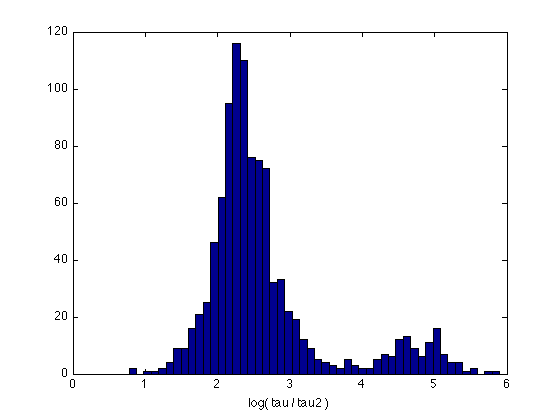
Descriptive statistics about the tau1-to-tau2 ratio
Take log of the time constants so that ratios become differences:
Representation scheme for "New 11-parameter model": X is a 1x11 vector: x(10) and x(11) store Tau and Tau2 for both groups
log_tau = log(B.optX(2:end,10:11)) ;             % [log_tau log_tau2]
log_tau = [log_tau, log_tau(:,1)-log_tau(:,2)] ; % [log_tau log_tau2, log_ratio]
describe(log_tau) ;
hist(log_tau(:,3),50) ; xlabel('log( tau / tau2 )') ;
st = exp(describe(log_tau))   % [mean std  min Q25 median Q75 max]

prctile(exp(log_tau(:,3)),[5 10 50 90 95])
    Mean  Std.dev       Min     Q25  Median     Q75     Max
------------------------------------------------------------
   7.258    0.375      6.09    7.01    7.27    7.50    8.64
   4.616    0.896      2.30    4.52    4.90    5.15    6.09
   2.642    0.858      0.78    2.18    2.40    2.76    5.90
------------------------------------------------------------
   4.839    0.710      3.06    4.57    4.86    5.14    6.88

st =

   1.0e+03 *

    1.4191    0.0015    0.4405    1.1120    1.4303    1.7994    5.6268
    0.1010    0.0025    0.0100    0.0918    0.1343    0.1728    0.4423
    0.0140    0.0024    0.0022    0.0088    0.0110    0.0158    0.3650


ans =

    5.5624    6.9321   11.0483   71.3121  121.7748
Explore 15-parameter model performance
fprintf('Alternative model: R2=%.4f  RMSE=%.4f\n',B.R2_alt(1),B.RMSE_alt(1)) ;
describe([B.R2_alt(2:end) B.RMSE_alt(2:end)]) ;
Alternative model: R2=0.9140  RMSE=0.0931

    Mean  Std.dev       Min     Q25  Median     Q75     Max
------------------------------------------------------------
   0.860    0.030      0.75    0.84    0.86    0.88    0.94
   0.129    0.014      0.10    0.12    0.13    0.14    0.19
------------------------------------------------------------
   0.495    0.022      0.42    0.48    0.50    0.51    0.56
Explore the parameters of the 15-parameter model
x = B.optX_alt(1,:) ;
par = job.problem_alt.vect2param(x) ;
fprintf('\nGroup:    Y1    Y2      Y3   Y18     Y19   Y24     Tau  Tau2 \n') ;
for k = 1:4
    p = par(k,:) ;
    fprintf('%s: %5.2f %5.2f   %5.2f %5.2f   %5.2f %5.2f   %5d %5d \n' ...
           ,G.descr{k} ...
           ,p(I.Y1),p(I.Y2), p(I.Y3),p(I.Y18), p(I.Y19),p(I.Y24)   ...
           ,round(p(I.Tau)), round(p(I.Tau2)) ) ;
end
fprintf('EzYxx/HdYxx = k = %.4f \n',x(indepGr_K_idx)) ;

describe(B.optX_alt(2:end,:)) ;

C = corrcoef(B.optX_alt(2:end,:)) ;
vn = job.problem_alt.vector_names ;
fprintf('\nCross-correlation matrix of parameters:') ;
for k=1:size(C,1)
    fprintf('\n%8s:',vn{k}) ;
    fprintf(' %5.2f',C(k,:)) ;
end
fprintf('\n\n') ;
Group:    Y1    Y2      Y3   Y18     Y19   Y24     Tau  Tau2
EzGr1:  1.02  1.33    1.26  2.03    1.17  1.68    1561   140
EzGr2:  1.07  1.39    1.26  1.85    1.80  1.83    1561   140
HdGr1:  0.76  0.98    0.93  1.50    0.87  1.25    1561   140
HdGr2:  0.79  1.03    0.93  1.37    1.33  1.35    1561   140
EzYxx/HdYxx = k = 1.3507

    Mean  Std.dev       Min     Q25  Median     Q75     Max
------------------------------------------------------------
   0.757    0.112      0.34    0.68    0.76    0.84    1.02
   0.987    0.063      0.78    0.94    0.99    1.03    1.20
   0.933    0.074      0.72    0.88    0.93    0.98    1.18
   1.509    0.186      0.87    1.39    1.51    1.64    2.10
   0.869    0.099      0.58    0.80    0.87    0.94    1.21
   1.251    0.096      0.87    1.19    1.25    1.31    1.52
   0.798    0.158      0.35    0.68    0.79    0.91    1.28
   1.033    0.137      0.66    0.93    1.03    1.12    1.50
   0.931    0.118      0.61    0.85    0.92    1.01    1.30
   1.365    0.106      1.06    1.29    1.36    1.44    1.66
   1.334    0.115      0.97    1.26    1.33    1.41    1.73
   1.354    0.137      1.00    1.26    1.35    1.44    1.73
   1.351    0.019      1.29    1.34    1.35    1.36    1.41
1685.414  639.776    430.51 1261.31 1581.79 1992.37 6017.22
 137.129   71.048     10.00   98.11  140.39  179.40  541.31
------------------------------------------------------------
 122.468   47.483     30.04   91.53  115.78  145.81  438.49

Cross-correlation matrix of parameters:
 HdGr1Y1:  1.00  0.38  0.37  0.34  0.46  0.30  0.01 -0.02 -0.04 -0.04 -0.01  0.01 -0.06 -0.17  0.03
 HdGr1Y2:  0.38  1.00  0.44  0.41  0.68  0.35  0.00 -0.01 -0.00 -0.02  0.03  0.02  0.14 -0.05 -0.48
 HdGr1Y3:  0.37  0.44  1.00  0.58  0.65  0.37 -0.02 -0.06 -0.03 -0.04 -0.03 -0.08 -0.14  0.11 -0.22
HdGr1Y18:  0.34  0.41  0.58  1.00  0.39  0.90  0.01 -0.01  0.11  0.09  0.01  0.00 -0.23  0.41  0.10
HdGr1Y19:  0.46  0.68  0.65  0.39  1.00  0.31  0.02  0.00  0.04 -0.01 -0.01  0.00  0.31  0.13 -0.12
HdGr1Y24:  0.30  0.35  0.37  0.90  0.31  1.00  0.05  0.05  0.16  0.15  0.00  0.06 -0.21  0.40  0.33
 HdGr2Y1:  0.01  0.00 -0.02  0.01  0.02  0.05  1.00  0.90  0.81  0.53  0.57  0.58  0.02 -0.23  0.07
 HdGr2Y2: -0.02 -0.01 -0.06 -0.01  0.00  0.05  0.90  1.00  0.86  0.75  0.62  0.75 -0.04 -0.31  0.12
 HdGr2Y3: -0.04 -0.00 -0.03  0.11  0.04  0.16  0.81  0.86  1.00  0.84  0.60  0.73 -0.13 -0.06  0.17
HdGr2Y18: -0.04 -0.02 -0.04  0.09 -0.01  0.15  0.53  0.75  0.84  1.00  0.46  0.72 -0.21 -0.06  0.18
HdGr2Y19: -0.01  0.03 -0.03  0.01 -0.01  0.00  0.57  0.62  0.60  0.46  1.00  0.77  0.04 -0.18 -0.09
HdGr2Y24:  0.01  0.02 -0.08  0.00  0.00  0.06  0.58  0.75  0.73  0.72  0.77  1.00 -0.30 -0.26  0.12
       k: -0.06  0.14 -0.14 -0.23  0.31 -0.21  0.02 -0.04 -0.13 -0.21  0.04 -0.30  1.00 -0.13 -0.24
     tau: -0.17 -0.05  0.11  0.41  0.13  0.40 -0.23 -0.31 -0.06 -0.06 -0.18 -0.26 -0.13  1.00  0.32
    tau2:  0.03 -0.48 -0.22  0.10 -0.12  0.33  0.07  0.12  0.17  0.18 -0.09  0.12 -0.24  0.32  1.00
Explore the raw specificity indices
fprintf('\nRaw data:        SI1=%s  SI2=%s\n' ...
       ,mat2str(raw_SI1,3),mat2str(raw_SI2,3)) ;
fprintf('Raw bootstrap:   SI1=%s  SI2=%s\n' ...
       ,mat2str(B.SI1_raw(1,:),3),mat2str(B.SI2_raw(1,:),3)) ;

fprintf('\nRaw specificity indices #1 and #2:') ;
SI = [B.SI1_raw(2:end,:) B.SI2_raw(2:end,:)] ;
vn = {'SI1_EzGr1' 'SI1_EzGr2' 'SI1_HdGr1' 'SI1_HdGr2' ...
     ,'SI2_EzGr1' 'SI2_EzGr2' 'SI2_HdGr1' 'SI2_HdGr2' } ;
describe(SI) ;

CI80 = prctile(SI,[10 50 90])' ;
fprintf('\n         :   P10   P50   P90 \n--------------------------------\n') ;
for k=1:size(CI80,1)
    fprintf('%9s: %5.2f %5.2f %5.2f \n',vn{k},CI80(k,1),CI80(k,2),CI80(k,3)) ;
end

C = corrcoef(SI) ;
fprintf('\n           :') ;
for k=1:size(C,1); fprintf(' %5d',k);end
for k=1:size(C,1)
    fprintf('\n%d %9s:',k,vn{k}) ;
    fprintf(' %5.2f',C(k,:)) ;
end
fprintf('\n\n') ;
Raw data:        SI1=[0.813 -0.0377 0.912 0.146]  SI2=[0.789 0.0937 0.886 0.343]
Raw bootstrap:   SI1=[0.813 -0.0377 0.912 0.146]  SI2=[0.789 0.0937 0.886 0.343]

Raw specificity indices #1 and #2:
    Mean  Std.dev       Min     Q25  Median     Q75     Max
------------------------------------------------------------
   0.822    0.189      0.29    0.70    0.80    0.92    2.66
  -0.074    0.245     -1.46   -0.19   -0.04    0.09    0.54
   0.916    0.219      0.11    0.78    0.89    1.03    1.95
   0.145    0.249     -0.65   -0.02    0.13    0.29    1.34
   0.791    0.210      0.10    0.66    0.78    0.91    1.78
  -0.291    6.056   -183.24   -0.16    0.12    0.28   11.22
   0.922    0.354     -0.47    0.71    0.87    1.04    3.48
   0.289    1.004    -12.52    0.17    0.35    0.50   23.19
------------------------------------------------------------
   0.440    1.066    -24.73    0.33    0.49    0.63    5.77

         :   P10   P50   P90
--------------------------------
SI1_EzGr1:  0.61  0.80  1.05
SI1_EzGr2: -0.40 -0.04  0.20
SI1_HdGr1:  0.68  0.89  1.18
SI1_HdGr2: -0.14  0.13  0.47
SI2_EzGr1:  0.54  0.78  1.05
SI2_EzGr2: -0.57  0.12  0.39
SI2_HdGr1:  0.58  0.87  1.29
SI2_HdGr2: -0.04  0.35  0.62

           :     1     2     3     4     5     6     7     8
1 SI1_EzGr1:  1.00  0.02  0.25 -0.00  0.87  0.07  0.25  0.00
2 SI1_EzGr2:  0.02  1.00  0.01  0.43  0.06  0.08  0.02  0.05
3 SI1_HdGr1:  0.25  0.01  1.00  0.02  0.20  0.15  0.86  0.05
4 SI1_HdGr2: -0.00  0.43  0.02  1.00  0.07  0.03  0.02  0.16
5 SI2_EzGr1:  0.87  0.06  0.20  0.07  1.00 -0.02  0.25 -0.07
6 SI2_EzGr2:  0.07  0.08  0.15  0.03 -0.02  1.00  0.05  0.16
7 SI2_HdGr1:  0.25  0.02  0.86  0.02  0.25  0.05  1.00  0.03
8 SI2_HdGr2:  0.00  0.05  0.05  0.16 -0.07  0.16  0.03  1.00
Explore the specificity indices under the New 11-parameter model
fprintf('11-param model:  SI1=%s  SI2=%s\n' ...
       ,mat2str(param11n_fit.specif_idx1(1:2),3) ...
       ,mat2str(param11n_fit.specif_idx2(1:2),3)) ;

fprintf('\nSpecificity indices #1 and #2 under the main model:') ;
SI = [B.SI1_main(2:end,1:2) B.SI2_main(2:end,1:2)] ;
vn = {'SI1_Gr1' 'SI1_Gr2' 'SI2_Gr1' 'SI2_Gr2'} ;
describe(SI) ;

CI80 = prctile(SI,[10 50 90])' ;
fprintf('\n         :   P10   P50   P90 \n--------------------------------\n') ;
for k=1:size(CI80,1)
    fprintf('%9s: %5.2f %5.2f %5.2f \n',vn{k},CI80(k,1),CI80(k,2),CI80(k,3)) ;
end

C = corrcoef(SI) ;
fprintf('\n           :') ;
for k=1:size(C,1); fprintf(' %5d',k);end
for k=1:size(C,1)
    fprintf('\n%d %9s:',k,vn{k}) ;
    fprintf(' %5.2f',C(k,:)) ;
end
fprintf('\n\n') ;
11-param model:  SI1=[0.877 0.0328]  SI2=[0.85 0.21]

Specificity indices #1 and #2 under the main model:
    Mean  Std.dev       Min     Q25  Median     Q75     Max
------------------------------------------------------------
   0.892    0.175      0.36    0.78    0.88    0.99    1.82
   0.004    0.179     -0.76   -0.10    0.02    0.13    0.42
   0.842    0.216     -0.09    0.72    0.84    0.99    1.63
   0.127    0.416     -3.45   -0.00    0.22    0.38    0.76
------------------------------------------------------------
   0.466    0.246     -0.99    0.35    0.49    0.62    1.16

         :   P10   P50   P90
--------------------------------
  SI1_Gr1:  0.69  0.88  1.11
  SI1_Gr2: -0.24  0.02  0.21
  SI2_Gr1:  0.58  0.84  1.12
  SI2_Gr2: -0.31  0.22  0.49

           :     1     2     3     4
1   SI1_Gr1:  1.00 -0.04  0.89 -0.28
2   SI1_Gr2: -0.04  1.00  0.05  0.27
3   SI2_Gr1:  0.89  0.05  1.00 -0.36
4   SI2_Gr2: -0.28  0.27 -0.36  1.00
Explore the specificity indices under the 15-parameter model
fprintf('15-param model:  SI1=%s  SI2=%s\n' ...
       ,mat2str(indepGr_cmnKTau_fit.specif_idx1(1:2),3) ...
       ,mat2str(indepGr_cmnKTau_fit.specif_idx2(1:2),3)) ;

fprintf('\nSpecificity indices #1 and #2 under the alternative model:') ;
SI = [B.SI1_alt(2:end,1:2) B.SI2_alt(2:end,1:2)] ;
vn = {'SI1_Gr1' 'SI1_Gr2' 'SI2_Gr1' 'SI2_Gr2'} ;
describe(SI) ;

CI80 = prctile(SI,[10 50 90])' ;
fprintf('\n         :   P10   P50   P90 \n--------------------------------\n') ;
for k=1:size(CI80,1)
    fprintf('%9s: %5.2f %5.2f %5.2f \n',vn{k},CI80(k,1),CI80(k,2),CI80(k,3)) ;
end

C = corrcoef(SI) ;
fprintf('\n           :') ;
for k=1:size(C,1); fprintf(' %5d',k);end
for k=1:size(C,1)
    fprintf('\n%d %9s:',k,vn{k}) ;
    fprintf(' %5.2f',C(k,:)) ;
end
fprintf('\n\n') ;
15-param model:  SI1=[0.856 0.0601]  SI2=[0.824 0.238]

Specificity indices #1 and #2 under the alternative model:
    Mean  Std.dev       Min     Q25  Median     Q75     Max
------------------------------------------------------------
   0.856    0.149      0.35    0.75    0.85    0.94    1.58
   0.033    0.227     -1.22   -0.08    0.05    0.18    0.66
   0.828    0.192      0.11    0.70    0.82    0.94    1.81
   0.081    1.766    -52.84    0.04    0.26    0.40    0.73
------------------------------------------------------------
   0.450    0.583    -13.40    0.35    0.50    0.62    1.20

         :   P10   P50   P90
--------------------------------
  SI1_Gr1:  0.67  0.85  1.04
  SI1_Gr2: -0.27  0.05  0.29
  SI2_Gr1:  0.61  0.82  1.05
  SI2_Gr2: -0.23  0.26  0.49

           :     1     2     3     4
1   SI1_Gr1:  1.00 -0.01  0.89  0.10
2   SI1_Gr2: -0.01  1.00  0.05  0.17
3   SI2_Gr1:  0.89  0.05  1.00 -0.01
4   SI2_Gr2:  0.10  0.17 -0.01  1.00