Contents
- MAESpec_diffusion_fits.m
- Load perceptual learning data
- Design parameters
- Load diffusion data, MODEL 1 and MODEL 2
- Load diffusion data, MODEL 3
- Compare the two fits of MODEL 3
- Load diffusion data, MODEL 4
- Compare the two fits of MODEL 4
- Define Learning index (LI) and Specificity index (SI)
- Segment the data and calculate specificity indices
- This for loop is old (prior to Oct 2010). It is updated for 11 periods
- Descriptive statistics for the chi-squares for the saturated model
- G-squared statistic per subject for each of the 4 models:
- Fix the anomalous G-square values for sbj 363, MODEL 1
- Bayesian Information Criterion (BIC)
- BIC competition outcomes counted across the 27 subjects
- Specificity Indices (for all sbjs averaged together)
- dprime confidence interval calculations
- RT confidence interval calculations
- diffusion confidence interval calculations
- Plot RT and RT std (sbjs averaged together)
- Plot dprime
- All subjects plot with separate deltas
- Plot diffusion params (averaged across all sbjs)
- Export data for the six-plot empirical figure, 2010-11-17
- Raw specificity values
- Diffusion paramter specificity values (avg across subjs)
- Bootstrap Specificity Indices and Confidence Intervals
- B(1) contains the SIs and LIs on the full data set
- Average over all N_samples to find more stable SI values
- Average over all N_samples to find more stable LI values
- Collect distribution statistics of the 11-point profiles
- Plot bootstrap dprime curve and SI value for single dprime
- Bootstrap-based dprime learning curves
- Plot the resulting diffusion param bootstrap curves with SI written below
- Ter analysis
- New diffusion models (2-4)
- Plot Bootstrap RT and RT std (sbjs averaged together)
- Raw bootstrap percentiles
- Descriptive statistics for the on-line supplement, 2010-07-14
- Specificity-index summary table
- Learning-index summary table
- Bootstrap group-level Z-tests about specificity indices, accuracy
- Bootstrap group-level Z-tests about Learning indices, accuracy
- Bootstrap group-level Z-tests comparing the indices for Ter and MeanRT
- Individual-level Learning indices, accuracy and drift rates
- Paired-sample t-tests of LIs, individual-subject data
- Proportionality of easy and hard d'
- Within-sbj ANOVA for the boundary separation parameter a
- Define linear and quadratic trend coefficients
- Linear trend analysis of boundary separation parameter a
- Quadratic trend analysis of boundary separation parameter a
- Linear (and quadratic) trend analysis of drift-stdev parameter eta
- Linear (and quadratic) trend analysis of starting-point range parameter sz
- Linear (and quadratic) trend analysis of easy drift rate v1
- Linear (and quadratic) trend analysis of difficult drift rate v2
- Linear (and quadratic) trend analysis of the average drift rate v_avg
- Linear (and quadratic) trend analysis of the average dprime
- Linear (and quadratic) trend analysis of the easy dprime
- Linear (and quadratic) trend analysis of the hard dprime
- Linear (and quadratic) trend analysis of the mean raw RT (sRT_all)
- Linear (and quadratic) trend analysis of mean nondecision time Ter
- Linear (and quadratic) trend analysis of nondecision-time range parameter st
- Linear (and quadratic) trend analysis of minimum nondecision time t1
- Linear (and quadratic) trend analysis of maximum nondecision time t2
- Bootstrap group-level Z-tests about boundary separation
- Bootstrap group-level Z-tests about nondecision times
- Descriptive statistics of the drop of the maximum nondecision time t2
- Descriptive statistics of the drop of the mean RT
MAESpec_diffusion_fits.m
Plot results of the diffusion-model analysis of MAESpec experiments
File: work/MLExper/MAESpec02/diffusion/MAESpec_diffusion_fits.m
Usage: publish('MAESpec_diffusion_fits.m','html') ;    %
'latex','doc','ppt'
% The following files will be created and re-used. To start fresh, these % files must first be deleted manually: % .../work/MLExper/MAESpec02/diffusion/H.mat (hitcount results) % .../work/MLExper/MAESpec02/diffusion/B.mat (bootstrap results) % (c) Laboratory for Cognitive Modeling and Computational Cognitive % Neuroscience at the Ohio State University, http://cogmod.osu.edu % % 1.4.5 2010-11-23 AAP -- Descriptive stats for the chi2 for the saturated model % 1.4.4 2010-11-17 AAP -- Export data for 6-panel Figure and Table 1 in PB&R % 1.4.3 2010-11-10 AAP -- Trend analyses for dprime and raw RTs % 1.4.2 2010-11-06 AAP -- diffusion_params_par11terb and ..._par11terstb % 1.4.1 2010-10-27 AAP -- G-squared and Bayesian Info Criterion (BIC) % 1.4.0 2010-10-22 AAP -- Trend analyses % 1.3.0 2010-10-18 NVH -- Added 3 d models. Forked script into 11-period version % 1.2.0 2010-07-06 AAP -- More z-tests. Learning indices % 1.1.1 2010-04-15 AAP -- z-tests instead of t-tests at the end % 1.1.0 2010-04-14 NVH -- Now includes SIs for the RTs, etc. % 1.0.0 2010-03-24 NVH -- Initial version
Load perceptual learning data
Raw subject data is loaded from .../work/MLEXper/MAESpec01/data & .../work/MLExper/MAESpec02/data
As of 2010-10-21: The stuff in this section is old. It is about d' and mean RTs. It generates H.mat, which is now stable.
cd(fullfile(MAESpec02_pathstr,'diffusion')) ;
fprintf('\n\nMAESpec_diffusion_fits executed on %s.\n\n',datestr(now)) ;
fprintf('cd %s\n',pwd) ;

clear all ;
filename = fullfile(MAESpec02_pathstr,'diffusion','H.mat') ;
%recalculatep = true ;
recalculatep = false ;
if (recalculatep || ~exist(filename,'file'))

    data_file = fullfile(MAESpec02_pathstr,'diffusion','raw_data.dat');
    if (~exist(data_file, 'file'))
        file_1 = fullfile(MAESpec01_pathstr,'data','sbj*.dat');
        file_2 = fullfile(MAESpec02_pathstr,'data','sbj*.dat');
        %- Concatenate the individual data files into one master ASCII file
        fprintf('!cat %s %s > %s \n', file_1, file_2, data_file) ;
        eval(['!cat ' file_1 ' ' file_2 ' > ' data_file]);
    end
    %- Import to Matlab
    fprintf('\nD=MAES02_import_data ...') ;
    D=MAES02_import_data(fullfile(MAESpec02_pathstr,'diffusion','raw_data.dat')) ;
    %- Calculate d-primes
    fprintf('\nH = MAES02_hitcount(D) ...\n') ;
    H = MAES02_hitcount(D) ;
    save(filename,'H') ;
    fprintf('\nsave %s \n\n',filename) ;
else
    fprintf('load %s \n\n',filename) ;
    load(filename) ;
end

N_sbj = length(H) ;
MAESpec_diffusion_fits executed on 29-Nov-2010 17:38:44.

cd /Users/apetrov/a/r/w/work/MLExper/MAESpec02/diffusion
load /Users/apetrov/a/r/w/work/MLExper/MAESpec02/diffusion/H.mat
Design parameters
These are fixed.
P = MAES02_params(0) ;
design_params = P.design_params ;
task_sched = design_params.task_sched ;         % 1=MAE, 2=discrim

N_sessions = design_params.N_session ;
N_discrim_sessions = N_sessions(2) ;                  % 5 sessions
N_MAE_sessions = N_sessions(1);                       % 2 sessions
MAE_blocks_session = design_params.blocks_session(1) ;     % 7 blocks per session
discrim_blocks_session = design_params.blocks_session(2) ; % 8 blocks per session
N_MAE_blocks = N_MAE_sessions * MAE_blocks_session ;
N_discrim_blocks = N_discrim_sessions * discrim_blocks_session ;
trials_MAE_block = design_params.trials_block(1) ;    % 12 trials per block
trials_discrim_block = design_params.trials_block(2) ;% 120 trials per block
N_MAE_trials = N_MAE_blocks * trials_MAE_block ;
N_discrim_trials = N_discrim_blocks * trials_discrim_block ;
Load diffusion data, MODEL 1 and MODEL 2
These data are described in .../work/MLExper/MAESpec02/diffusion/diffusion_params.txt
As of 2010-10-21, this is a fully saturated DM fit in which all params are allowed to vary for each period and each subject. One period is half-day's worth (4 blocks in MAESpec01_params terminology), except period 9, which is the "rogue block" immediately after the second MAE session. See blocks_per_period = [4 4 4 4 4 4 4 4 1 4 3] below. In later sections, this diffusion model fit is implicitly referred to as MODEL_1. Whenever there is something with no explicit subscript, it should be implicitly understood that the subscript is 1.
N_periods_total = 11 ;   % as of 2010-10-18

df_1 = load(fullfile(MAESpec02_pathstr, 'diffusion', 'diffusion_params.txt'), '-ascii');
assert(all(size(df_1)==[N_sbj*N_periods_total 11])) ;


% Load the new diffusion models (requested by reviewers)
% As of 2010-10-21, these are MODEL_2, MODEL_3, and MODEL_4, as follows:
% ** MODEL_2 is what Roger labeled 'par11a' in his email of 2010-10-09.
%    In MODEL_2, only drift is allowed to vary across periods. The same
%    boundary separation a and the same Ter and st apply across the board
%    for each individual subject.
df_2 = load(fullfile(MAESpec02_pathstr, 'diffusion', 'diffusion_params_par11a.txt'), '-ascii');
assert(all(size(df_2)==[N_sbj 31])) ;
Load diffusion data, MODEL 3
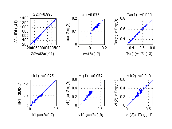
** MODEL_3 is what Roger labeled 'par11tera' in his email of 2010-10-09. A second parameter search from a different starting point was performed on 2010-10-30 and emailed as 'par11terb'. In MODEL_3, both drift and Ter are allowed to vary across periods. The same boundary separation a and the same st apply across the board for each individual subject.
df_3a = load(fullfile(MAESpec02_pathstr, 'diffusion', 'diffusion_params_par11tera.txt'), '-ascii');
assert(all(size(df_3a)==[N_sbj 41])) ;

df_3b = load(fullfile(MAESpec02_pathstr, 'diffusion', 'diffusion_params_par11terb.txt'), '-ascii');
assert(all(size(df_3b)==[N_sbj 40])) ;

% Bring the two versions to a common data format
df_3b = [df_3a(:,1) , df_3b] ;   % append sbj_number as column 1

% The G-squared statistic (column 41) must be multiplied by 2 in par11tera
% per Roger's email of 2010-10-27.  The G^2 formula was corrected by the
% time (2010-10-30) that par11terb was produced.
% See Roger & Smith (2004, Psych Review, vol 111, equation on p. 343)
df_3a(:,41) = df_3a(:,41).*2 ;
Compare the two fits of MODEL 3
idx = [41 2 3 7 9 11] ;
name = {'G2', 'a', 'Ter(1)', 'st(1)', 'v1(1)', 'v1(2)'} ;
ax = {[200 1400], [0 .2], [.300 .800], [0 .5], [0 .6], [0 .6]} ;

clf ;
for k = idx
    kk = find(idx==k) ;
    subplot(2,3,kk) ;
    plot(df_3a(:,k),df_3b(:,k),'.');
    axis([ax{kk} ax{kk}]) ; axis square ;
    refline(1,0); grid on;
    xlabel(sprintf('%s=df3a(:,%d)',name{kk},k));
    ylabel(sprintf('%s=df3b(:,%d)',name{kk},k));
    title(sprintf('%s: r=%.3f',name{kk},corr(df_3a(:,k),df_3b(:,k)))) ;
end

describe(df_3a(:,idx)-df_3b(:,idx),name) ;

% As the second run [df_3b=par11terb] yields lower G^2 values for all
% subjects, we'll adopt it for all subsequent calculations:
df_3 = df_3b ;
assert(all(df_3(:,41)<=df_3a(:,41))) ;
assert(all(df_3(:,41)<=df_3b(:,41))) ;

clear k name ax kk idx name
    Mean  Std.dev       Min     Q25  Median     Q75     Max
------------------------------------------------------------
  20.713   24.235      1.27    4.14   12.38   24.69   98.88  G2
  -0.002    0.005     -0.01   -0.01   -0.00   -0.00    0.01  a
  -0.003    0.005     -0.01   -0.01   -0.00    0.00    0.01  Ter(1)
   0.000    0.012     -0.03   -0.01   -0.00    0.01    0.03  st(1)
  -0.018    0.020     -0.07   -0.03   -0.01   -0.01    0.02  v1(1)
  -0.015    0.025     -0.08   -0.02   -0.01   -0.00    0.03  v1(2)
------------------------------------------------------------
   3.446    4.050      0.18    0.68    2.06    4.11   16.50
Load diffusion data, MODEL 4
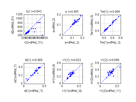
** MODEL_4 is what Roger labeled 'par11tersta' in his email of 2010-10-09. A second parameter search from a different starting point was performed on 2010-10-30 and emailed as 'par11terstb'. In MODEL_4, three things (4 parameters total because there is easy and hard drift) are allowed to vary across periods. These are: - drift rate (easy and hard) - mean nondecision time Ter - range of the nondecision time distribution st The same boundary separation a applies across the board for each individual subject. Also the same eta and sz.
df_4a = load(fullfile(MAESpec02_pathstr, 'diffusion', 'diffusion_params_par11tersta.txt'), '-ascii');
assert(all(size(df_4a)==[N_sbj 51])) ;

df_4b = load(fullfile(MAESpec02_pathstr, 'diffusion', 'diffusion_params_par11terstb.txt'), '-ascii');
assert(all(size(df_4b)==[N_sbj 50])) ;

% Bring the two versions to a common data format
df_4b = [df_4a(:,1) , df_4b] ;   % append sbj_number as column 1

% The G-squared statistic (column 51) must be multiplied by 2 in par11tersta
% per Roger's email of 2010-10-27.  The G^2 formula was corrected by the
% time (2010-10-30) that par11terstb was produced.
% See Roger & Smith (2004, Psych Review, vol 111, equation on p. 343)
df_4a(:,51) = df_4a(:,51).*2 ;
Compare the two fits of MODEL 4
idx = [51 2 3 7 9 11] ;
name = {'G2', 'a', 'Ter(1)', 'st(1)', 'v1(1)', 'v1(2)'} ;
ax = {[200 1200], [0 .2], [.300 .800], [0 .5], [0 .6], [0 .6]} ;

clf ;
for k = idx
    kk = find(idx==k) ;
    subplot(2,3,kk) ;
    plot(df_4a(:,k),df_4b(:,k),'.');
    axis([ax{kk} ax{kk}]) ; axis square ;
    refline(1,0); grid on;
    xlabel(sprintf('%s=df4a(:,%d)',name{kk},k));
    ylabel(sprintf('%s=df4b(:,%d)',name{kk},k));
    title(sprintf('%s: r=%.3f',name{kk},corr(df_4a(:,k),df_4b(:,k)))) ;
end

describe(df_4a(:,idx)-df_4b(:,idx),name) ;

% The fits aren't very stable.  Among the two parameter sets for each
% subject, take the one that yields lower G^2.  Note that there is no
% guarantee that this is the global minimum.  In his email of 2010-10-30,
% Roger writes:
% "Some of the drift rates had not stabilized even after 7000 iterations.
%  This was the largest number of drift rates fit in one program..."
df_4 = df_4b ;
idx = find(df_4(:,51)>df_4a(:,51)) ;
df_4(idx,:) = df_4a(idx,:) ;

df_4b(idx,[1 51]) % plot the subject numbers for whom the old fit was better

assert(all(df_4(:,51)<=df_4a(:,51))) ;
assert(all(df_4(:,51)<=df_4b(:,51))) ;

clear k name ax kk idx name
    Mean  Std.dev       Min     Q25  Median     Q75     Max
------------------------------------------------------------
  89.133  176.762    -16.16   15.03   34.61   82.42  883.65  G2
  -0.002    0.010     -0.03   -0.01    0.00    0.00    0.02  a
  -0.005    0.012     -0.03   -0.01   -0.00    0.00    0.02  Ter(1)
  -0.013    0.027     -0.06   -0.03   -0.01    0.00    0.09  st(1)
  -0.015    0.037     -0.10   -0.04   -0.01    0.01    0.04  v1(1)
  -0.010    0.057     -0.12   -0.05   -0.01    0.02    0.16  v1(2)
------------------------------------------------------------
  14.848   29.484     -2.75    2.48    5.76   13.74  147.33

ans =

  356.0000  285.9980
  362.0000  347.5690
Define Learning index (LI) and Specificity index (SI)
Input is a m-by-11 matrix of profiles. Output a m-by-1 vector of indices
assert(N_periods_total==11) ;   % as of 2010-10-18
N_periods_train = 8 ;    % 4 training sessions, each split in half

%-- Learning index (LI) -- similar (but not identical) to that of Fine & Jacobs (2002)
learn_idx = @(x) ((x(:,8)-x(:,1)) ./ x(:,1)) ;

%-- Specificity index (SI) -- Ahissar & Hochstein (1997)
specif_idx = @(x) ((x(:,8)-x(:,10)) ./ (x(:,8)-x(:,1))) ;
Segment the data and calculate specificity indices
These are all up-to-date as of 2010-10-21 -- all geared for 11 time periods
%[r,c] = recommend_subplot_size(N_sbj) ;
r = 1;
c = 2;
M = 4.5 ;
start_block = 4 ;
end_block = 55 ;

% Matrix of each subject's dprime and diffusion means for the 11 "blocks" of
% interest
% 1 row per sbj. 110 columns = dprime 1:11, then 11 columns per diffusion
% parameter. Columns =
%           dprime; a; Ter; eta; sz; st; v1; v2
% followed by 11 columns of easy dprime and 11 columns of hard dprime
sbj_means = NaN(N_sbj, 110) ;

% G-squared goodness-of-fit statistic
% See Roger & Smith (2004, Psych Review, vol 111, equation on p. 343)
Gsq_1_per_period = NaN(N_sbj,N_periods_total) ;  % G-squared for MODEL 1

% Matrix of specificty indices
SI = NaN(N_sbj, N_periods_train) ;    % using session 8 as the final day of training
SIb = NaN(N_sbj, N_periods_train) ;   % using session 8, block 1 as the final day of training
SIc = NaN(N_sbj, N_periods_train) ;   % using session 8, block 1 as the first day of *transfer*

% Preallocate indv subject RT matrix
sRT_all = NaN(N_sbj, N_periods_total) ;
sRT_corr = NaN(N_sbj, N_periods_total) ;    % RTs for correct trials only
RTsd_all = NaN(N_sbj, N_periods_total) ;
RTsd_corr = NaN(N_sbj, N_periods_total) ;


%%%%%%%%%%%%%%%%%%%%%%%
%%%%%%%%%%%%%%%%%%%%%%%
%
% Define indices so that so params can be called by name

% These indices are relevant for MODEL_1
assert(N_periods_total==11) ;
dpr = 1:11;
a = 12:22;
ter = 23:33;
eta = 34:44;
sz = 45:55;
st = 56:66;
v1 = 67:77;
v2 = 78:88;
edpr_idx = 89:99;
hdpr_idx = 100:110;


% 2010-10-20: The data layout of the various files that Roger emailed to us
% over a period of several months is different. Thus, we need a separate
% set of indices for each.
% 2010-10-20: Define indices for the new diffusion MODELs 2 through 4.

% These indices are relevant for MODEL_2
a_2 = 2 ;
ter_2 = 3 ;
eta_2 = 4 ;
sz_2 = 5 ;
st_2 = 7 ;
v1_2 = 9:2:29 ;
v2_2 = 10:2:30 ;
gsq_2 = 31 ; % g squared value

% These indices are relevant for MODEL_3
a_3 = 2 ;
ter_3 = [3 31:40] ;
eta_3 = 4 ;
sz_3 = 5 ;
st_3 = 7 ;
v1_3 = 9:2:29 ;
v2_3 = 10:2:30 ;
gsq_3 = 41 ; % g squared value

% These indices are relevant for MODEL_4
a_4 = 2 ;
ter_4 = [3 31:40] ;
eta_4 = 4 ;
sz_4 = 5 ;
st_4 = [7 41:50];
v1_4 = 9:2:29 ;
v2_4 = 10:2:30 ;
gsq_4 = 51 ; % g squared value
This for loop is old (prior to Oct 2010). It is updated for 11 periods
now (there used to be only 8 periods in the manuscript submitted to PBR
on 2010-08-03). It is mostly about packaging, calculating means, and
plotting d' and RTs.
for k=1:N_sbj
    % Average easy and hard dprime data into 11 periods like the
    % duffusion results. 4 blocks per period, except periods 9 & 11
dp11 = [mean(H(k).all_dprime(1:4))...   % Session 1 (1/2)
        mean(H(k).all_dprime(5:8))...     % Session 1 (2/2)
        mean(H(k).all_dprime(9:12))...     % Session 2 (1/2) ...
        mean(H(k).all_dprime(13:16))...     % Session 2 (2/2) ...
        mean(H(k).all_dprime(17:20))...     % Session 3 (1/2) ...
        mean(H(k).all_dprime(21:24))...     % Session 3 (2/2)
        mean(H(k).all_dprime(25:28))...     % Session 4 (1/2) ...
        mean(H(k).all_dprime(29:32))...     % Session 4 (2/2)
        mean(H(k).all_dprime(33))...        % Session 5 *block 1* (1/3)
        mean(H(k).all_dprime(34:37))...     % Session 5 (2/3)
        mean(H(k).all_dprime(38:40))];      % Session 5 (3/3)

    edp11 = [mean(H(k).easy_dprime(1:4))...   % Session 1 (1/2)
        mean(H(k).easy_dprime(5:8))...     % Session 1 (2/2)
        mean(H(k).easy_dprime(9:12))...     % Session 2 (1/2) ...
        mean(H(k).easy_dprime(13:16))...     % Session 2 (2/2)
        mean(H(k).easy_dprime(17:20))...     % Session 3 (1/2) ...
        mean(H(k).easy_dprime(21:24))...     % Session 3 (2/2)
        mean(H(k).easy_dprime(25:28))...     % Session 4 (1/2) ...
        mean(H(k).easy_dprime(29:32))...     % Session 4 (2/2)
        mean(H(k).easy_dprime(33))...        % Session 5 *block 1* (1/3)
        mean(H(k).easy_dprime(34:37))...     % Session 5 (2/3)
        mean(H(k).easy_dprime(38:40))];      % Session 5 (3/3)
    hdp11 = [mean(H(k).hard_dprime(1:4))...   % Session 1 (1/2)
        mean(H(k).hard_dprime(5:8))...     % Session 1 (2/2)
        mean(H(k).hard_dprime(9:12))...     % Session 2 (1/2) ...
        mean(H(k).hard_dprime(13:16))...     % Session 2 (2/2)
        mean(H(k).hard_dprime(17:20))...     % Session 3 (1/2) ...
        mean(H(k).hard_dprime(21:24))...     % Session 3 (2/2)
        mean(H(k).hard_dprime(25:28))...     % Session 4 (1/2) ...
        mean(H(k).hard_dprime(29:32))...     % Session 4 (2/2)
        mean(H(k).hard_dprime(33))...        % Session 5 *block 1* (1/3)
        mean(H(k).hard_dprime(34:37))...     % Session 5 (2/3)
        mean(H(k).hard_dprime(38:40))];      % Session 5 (3/3)

    % Collect RT statistics
    % Mean RT (of *median* block RTs)
    sRT_all(k,:) = [mean(H(k).RT_descr(1:4,5),1)...   % Session 1 (1/2)
        mean(H(k).RT_descr(5:8,5),1)...     % Session 1 (2/2)
        mean(H(k).RT_descr(9:12,5),1)...     % Session 2 (1/2) ...
        mean(H(k).RT_descr(13:16,5),1)...     % Session 2 (2/2)
        mean(H(k).RT_descr(17:20,5),1)...     % Session 3 (1/2) ...
        mean(H(k).RT_descr(21:24,5),1)...     % Session 3 (2/2)
        mean(H(k).RT_descr(25:28,5),1)...     % Session 4 (1/2) ...
        mean(H(k).RT_descr(29:32,5),1)...     % Session 4 (2/2)
        mean(H(k).RT_descr(33,5),1)...        % Session 5 *block 1* (1/3)
        mean(H(k).RT_descr(34:37,5),1)...     % Session 5 (2/3)
        mean(H(k).RT_descr(38:40,5),1)];      % Session 5 (3/3)

    sRT_corr(k,:) = [mean(H(k).RT_descr_corr(1:4,5),1)...   % Session 1 (1/2)
        mean(H(k).RT_descr_corr(5:8,5),1)...     % Session 1 (2/2)
        mean(H(k).RT_descr_corr(9:12,5),1)...     % Session 2 (1/2) ...
        mean(H(k).RT_descr_corr(13:16,5),1)...     % Session 2 (2/2)
        mean(H(k).RT_descr_corr(17:20,5),1)...     % Session 3 (1/2) ...
        mean(H(k).RT_descr_corr(21:24,5),1)...     % Session 3 (2/2)
        mean(H(k).RT_descr_corr(25:28,5),1)...     % Session 4 (1/2) ...
        mean(H(k).RT_descr_corr(29:32,5),1)...     % Session 4 (2/2)
        mean(H(k).RT_descr_corr(33,5),1)...        % Session 5 *block 1* (1/3)
        mean(H(k).RT_descr_corr(34:37,5),1)...     % Session 5 (2/3)
        mean(H(k).RT_descr_corr(38:40,5),1)];      % Session 5 (3/3)

    % std of RT across "blocks"
    RTsd_all(k,:) = [mean(H(k).RT_descr(1:4,2),1)...   % Session 1 (1/2)
        mean(H(k).RT_descr(5:8,2),1)...     % Session 1 (2/2)
        mean(H(k).RT_descr(9:12,2),1)...     % Session 2 (1/2) ...
        mean(H(k).RT_descr(13:16,2),1)...     % Session 2 (2/2)
        mean(H(k).RT_descr(17:20,2),1)...     % Session 3 (1/2) ...
        mean(H(k).RT_descr(21:24,2),1)...     % Session 3 (2/2)
        mean(H(k).RT_descr(25:28,2),1)...     % Session 4 (1/2) ...
        mean(H(k).RT_descr(29:32,2),1)...     % Session 4 (2/2)
        mean(H(k).RT_descr(33,2),1)...        % Session 5 *block 1* (1/3)
        mean(H(k).RT_descr(34:37,2),1)...     % Session 5 (2/3)
        mean(H(k).RT_descr(38:40,2),1)];      % Session 5 (3/3)

    RTsd_corr(k,:) = [mean(H(k).RT_descr_corr(1:4,2),1)...   % Session 1 (1/2)
        mean(H(k).RT_descr_corr(5:8,2),1)...     % Session 1 (2/2)
        mean(H(k).RT_descr_corr(9:12,2),1)...     % Session 2 (1/2) ...
        mean(H(k).RT_descr_corr(13:16,2),1)...     % Session 2 (2/2)
        mean(H(k).RT_descr_corr(17:20,2),1)...     % Session 3 (1/2) ...
        mean(H(k).RT_descr_corr(21:24,2),1)...     % Session 3 (2/2)
        mean(H(k).RT_descr_corr(25:28,2),1)...     % Session 4 (1/2) ...
        mean(H(k).RT_descr_corr(29:32,2),1)...     % Session 4 (2/2)
        mean(H(k).RT_descr_corr(33,2),1)...        % Session 5 *block 1* (1/3)
        mean(H(k).RT_descr_corr(34:37,2),1)...     % Session 5 (2/3)
        mean(H(k).RT_descr_corr(38:40,2),1)];      % Session 5 (3/3)

    % Store sbj dprime means
    sbj_means(k, dpr) = dp11 ;

    % Isolate diffusion params for the current subject
    idx = find(df_1(:,1)==H(k).sbj) ;

    % sanity check
    current_sbj = H(k).sbj ;
    assert(all(df_1(idx,1)==current_sbj)) ;
    assert(df_2(k,1)==current_sbj) ;
    assert(df_2(k,1)==current_sbj) ;
    assert(df_2(k,1)==current_sbj) ;

    % param "a"
    sbj_means(k,a) = df_1(idx, 2)';
    % param "Ter"
    sbj_means(k,ter) = df_1(idx, 3)';
    % param "eta"
    sbj_means(k,eta) = df_1(idx, 4)';
    % param "sz"
    sbj_means(k,sz) = df_1(idx, 5)';
    % param "st"
    sbj_means(k,st) = df_1(idx, 7)';
    % param "v1"
    sbj_means(k,v1) = -df_1(idx, 9)';
    % param "v2"
    sbj_means(k,v2) = -df_1(idx, 10)';
    % G-squared goodness-of-fit statistic
    Gsq_1_per_period(k,:) = df_1(idx,11)' ;

    % easy dprime
    sbj_means(k,edpr_idx) = edp11 ;
    % difficult dprime
    sbj_means(k,hdpr_idx) = hdp11 ;

    % Easy/Hard specificity indices for plotting
    %e_SI = (edp8(5) - edp8(7)) / (edp8(5) - edp8(1)) ;
    %h_SI = (hdp8(5) - hdp8(7)) / (hdp8(5) - hdp8(1)) ;
    e_SI = specif_idx(edp11) ;
    h_SI = specif_idx(hdp11) ;

    % Specificity Indices using session 4 as final "block" of training data
    SI(k, :) = [
        (sbj_means(k,dpr(8))-sbj_means(k,dpr(10)))/(sbj_means(k,dpr(8))-sbj_means(k,dpr(1))),...
        (sbj_means(k,a(8))-sbj_means(k,a(10)))/(sbj_means(k,a(8))-sbj_means(k,a(1))),...
        (sbj_means(k,ter(8))-sbj_means(k,ter(10)))/(sbj_means(k,ter(8))-sbj_means(k,ter(1))),...
        (sbj_means(k,eta(8))-sbj_means(k,eta(10)))/(sbj_means(k,eta(8))-sbj_means(k,eta(1))),...
        (sbj_means(k,sz(8))-sbj_means(k,sz(10)))/(sbj_means(k,sz(8))-sbj_means(k,sz(1))),...
        (sbj_means(k,st(8))-sbj_means(k,st(10)))/(sbj_means(k,st(8))-sbj_means(k,st(1))),...
        (sbj_means(k,v1(8))-sbj_means(k,v1(10)))/(sbj_means(k,v1(8))-sbj_means(k,v1(1))),...
        (sbj_means(k,v2(8))-sbj_means(k,v2(10)))/(sbj_means(k,v2(8))-sbj_means(k,v2(1)))] ;
    SIb(k, :) = [
        (sbj_means(k,dpr(9))-sbj_means(k,dpr(10)))/(sbj_means(k,dpr(9))-sbj_means(k,dpr(1))),...
        (sbj_means(k,a(9))-sbj_means(k,a(10)))/(sbj_means(k,a(9))-sbj_means(k,a(1))),...
        (sbj_means(k,ter(9))-sbj_means(k,ter(10)))/(sbj_means(k,ter(9))-sbj_means(k,ter(1))),...
        (sbj_means(k,eta(9))-sbj_means(k,eta(10)))/(sbj_means(k,eta(9))-sbj_means(k,eta(1))),...
        (sbj_means(k,sz(9))-sbj_means(k,sz(10)))/(sbj_means(k,sz(9))-sbj_means(k,sz(1))),...
        (sbj_means(k,st(9))-sbj_means(k,st(10)))/(sbj_means(k,st(9))-sbj_means(k,st(1))),...
        (sbj_means(k,v1(9))-sbj_means(k,v1(10)))/(sbj_means(k,v1(9))-sbj_means(k,v1(1))),...
        (sbj_means(k,v2(9))-sbj_means(k,v2(10)))/(sbj_means(k,v2(9))-sbj_means(k,v2(1)))] ;
    SIc(k, :) = [
        (sbj_means(k,dpr(8))-sbj_means(k,dpr(9)))/(sbj_means(k,dpr(8))-sbj_means(k,dpr(1))),...
        (sbj_means(k,a(8))-sbj_means(k,a(9)))/(sbj_means(k,a(8))-sbj_means(k,a(1))),...
        (sbj_means(k,ter(8))-sbj_means(k,ter(9)))/(sbj_means(k,ter(8))-sbj_means(k,ter(1))),...
        (sbj_means(k,eta(8))-sbj_means(k,eta(9)))/(sbj_means(k,eta(8))-sbj_means(k,eta(1))),...
        (sbj_means(k,sz(8))-sbj_means(k,sz(9)))/(sbj_means(k,sz(8))-sbj_means(k,sz(1))),...
        (sbj_means(k,st(8))-sbj_means(k,st(9)))/(sbj_means(k,st(8))-sbj_means(k,st(1))),...
        (sbj_means(k,v1(8))-sbj_means(k,v1(9)))/(sbj_means(k,v1(8))-sbj_means(k,v1(1))),...
        (sbj_means(k,v2(8))-sbj_means(k,v2(9)))/(sbj_means(k,v2(8))-sbj_means(k,v2(1)))] ;

%     % Plot dprime
%     subplot(r,c,1) ;
%     plot(1:11, edp11,'b.-') ;
%     hold on
%     plot(1:11, hdp11, 'r.-') ;
%     axis([1 11 0 M]) ; grid on ;
%     set(gca,'xtick',([1:11]),...
%         'xticklabel',[],'ytick',(0:ceil(M))) ;
%     title(sprintf('Sbj %d, gr %d',H(k).sbj,H(k).group)) ;
%     ylabel('dprime');
%     xlabel(sprintf('SI(e) = %0.3f ; SI(h) = %0.3f', e_SI, h_SI));
%     hold off
%
%     % Plot drift rates
%     subplot(r,c,2) ;
%     plot(1:11, sbj_means(k,v1), 'b.-');
%     hold on
%     plot(1:11, sbj_means(k,v2), 'r.-');
%     axis([1 11 0 1]) ; grid on ;
%     set(gca,'xtick',([1:11]),...
%         'xticklabel',[],'ytick',(0:.1:1)) ;
%     title(sprintf('Sbj %d, gr %d',H(k).sbj,H(k).group)) ;
%     ylabel('drift rate');
%     xlabel(sprintf('SI(v1) = %0.3f ; SI(v2) = %0.3f', SI(k,7), SI(k,8)));
%     legend('v1','v2','location','NorthEast');
%     hold off
end
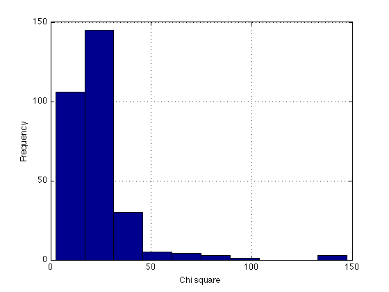
Descriptive statistics for the chi-squares for the saturated model
Added by Alex, 2010-11-23:
When Roger did his original fit (MODEL 1), he used ordinary chi-square to evaluate the goodness of fit. Then he switched to Gsq for Models 2, 3, and 4. The motivation for this was that Gsq is the mathematically appropriate term for the BIC calculation. Both are asymptotically distributed as chi-square with the same df. However, MODEL 1 (the saturated model) was never re-fit to optimize Gsq instead of chi2.
This is just as well because in the final manuscript we decided to stick to Model 1 (given that most parameters had statistically significant learning trends) and to report the standard chi-squared measure of fit.
%- Goodness-of-fit measure for the diffusion model
%  Chi-square values, as per Roger's email of 2010-01-19.
%  The 6-parameter DDM (z=a/2) was fit to individual data in each period,
%  after which the parameter values (and the chi-squares?) were averaged
%  across Ss to yield the following:

chi2=[38.185 27.154 27.034 22.644 24.842 15.799 18.845 19.900] ;

fprintf('\n Chi2 per Roger''s email: summed across blocks:') ;
describe(chi2,'chi2')

% This is close to the critical chi2=25.0=chi2inv(.95,15) % df=15, alpha=5%
% This indicates excellent fits -- most of the discrepancy between model
% and data can be attributed to sampling fluctuations.

critical_chi2 = chi2inv(.95,15)


%- Calculated from the imported DM fits: summed across Ss, varies across blocks
block_legend = cell(N_periods_total,1) ;

fprintf('\n Chi2 for saturated model: summed across Ss, varies across blocks:') ;
for k=1:N_periods_total ; block_legend{k} = sprintf('Block %2d',k) ; end

describe(Gsq_1_per_period,block_legend) ;    % summed across all Ss


%- Calculated from the imported DM fits: summed across blocks, varies across Ss
sbj_legend = cell(N_sbj,1) ;

fprintf('\n Chi2 for saturated model: summed across blocks, varies across Ss:') ;
for k=1:N_sbj ; sbj_legend{k} = sprintf('Sbj %3d',H(k).sbj) ; end

describe(Gsq_1_per_period',sbj_legend) ;    % summed across all blocks


%- Summed across everything
fprintf('\n Chi2 for saturated model: summed across both Ss and blocks:') ;
describe(Gsq_1_per_period(:)) ;

clf ;
hist(Gsq_1_per_period(:)) ; grid on
xlabel('Chi square') ; ylabel('Frequency') ;


% Number of significant deviations
k = Gsq_1_per_period>critical_chi2 ;   % [N_sbj x N_periods_total]

fprintf('\n Number of significant chi2 in each block:\n %s \n' ...
       ,mat2str(sum(k))) ;

fprintf('\n Number of significant chi2 in each subject:\n %s \n' ...
       ,mat2str(sum(k,2)')) ;

fprintf('\n Total number of significant chi2: %d out of %d \n'...
       ,sum(k(:)), length(k(:))) ;


% Number of large deviations
acceptable_chi2 = 2*critical_chi2
k = Gsq_1_per_period>acceptable_chi2 ;   % [N_sbj x N_periods_total]

fprintf('\n Number of unacceptable chi2 in each block:\n %s \n' ...
       ,mat2str(sum(k))) ;

fprintf('\n Number of unacceptable chi2 in each subject:\n %s \n' ...
       ,mat2str(sum(k,2)')) ;

fprintf('\n Total number of unacceptable chi2: %d out of %d \n'...
       ,sum(k(:)), length(k(:))) ;

k = sort(Gsq_1_per_period(:),'descend')' ;
fprintf('\n The ten most deviating values:\n %s \n', mat2str(k(1:10))) ;

clear k ;
 Chi2 per Roger's email: summed across blocks:
    Mean  Std.dev       Min     Q25  Median     Q75     Max
------------------------------------------------------------
  24.300    6.895     15.80   19.37   23.74   27.09   38.19  chi2

critical_chi2 =

   24.9958


 Chi2 for saturated model: summed across Ss, varies across blocks:
    Mean  Std.dev       Min     Q25  Median     Q75     Max
------------------------------------------------------------
  36.115   34.193     10.63   18.05   22.46   30.38  141.71  Block  1
  26.342   10.846      9.96   18.63   23.07   33.94   48.92  Block  2
  23.645    9.965      9.22   15.46   21.83   30.17   52.82  Block  3
  29.842   30.234      6.42   16.13   20.48   29.43  147.43  Block  4
  23.272   12.604      9.90   16.80   21.78   26.81   77.81  Block  5
  23.610   13.615      3.27   14.11   21.48   30.74   70.72  Block  6
  19.757    7.572      8.24   14.28   18.38   23.59   38.66  Block  7
  24.772   15.879      4.54   13.94   20.51   31.76   72.70  Block  8
  14.760    5.833      4.94   10.44   13.89   20.55   23.91  Block  9
  18.378    8.444      2.46   13.08   15.89   22.81   37.08  Block 10
  19.295    7.834      5.58   14.50   18.59   22.10   40.73  Block 11
------------------------------------------------------------
  23.617   14.274      6.83   15.04   19.85   27.48   68.41

 Chi2 for saturated model: summed across blocks, varies across Ss:
    Mean  Std.dev       Min     Q25  Median     Q75     Max
------------------------------------------------------------
  24.320   11.509     10.91   15.43   21.40   33.28   46.90  Sbj 353
  18.705   10.997      4.54    9.71   16.60   26.54   39.62  Sbj 354
  21.325    7.710     11.43   15.75   19.04   27.60   35.27  Sbj 355
  19.514    6.806     12.05   13.79   17.14   26.48   30.55  Sbj 356
  25.630   21.531     11.19   14.10   18.56   21.89   86.32  Sbj 357
  19.198    8.293      2.46   15.03   19.68   22.20   33.89  Sbj 359
  40.724   40.957      9.22   14.22   28.24   45.88  141.71  Sbj 360
  22.261   10.735     10.42   14.49   19.42   27.64   41.39  Sbj 362
  34.154   28.968      4.94   14.37   20.41   62.80   81.65  Sbj 363
  21.709    8.907      7.24   16.96   21.41   30.33   34.68  Sbj 364
  17.953    6.609      6.42   13.53   18.22   21.49   28.48  Sbj 366
  21.412    7.116     10.97   14.52   23.41   27.59   29.74  Sbj 367
  24.616    6.135     15.50   21.10   22.98   28.88   36.05  Sbj 382
  18.997    8.426      9.49   12.21   17.05   24.50   35.10  Sbj 383
  16.155    4.581      6.68   14.22   14.89   19.98   23.23  Sbj 384
  27.555    9.524     15.14   19.57   25.55   33.98   45.02  Sbj 385
  18.793    5.862      9.11   15.14   18.20   24.48   26.23  Sbj 386
  32.301   38.845     10.64   14.35   20.53   28.28  147.43  Sbj 387
  21.584    9.534      9.71   12.47   22.09   25.71   42.10  Sbj 388
  19.541    8.291      9.96   14.06   18.46   23.47   37.08  Sbj 389
  30.981   22.691      8.59   16.49   20.73   51.28   70.72  Sbj 390
  32.625   34.764     11.41   18.07   24.49   29.29  135.67  Sbj 391
  28.329   11.476     17.14   18.83   21.49   38.66   48.06  Sbj 392
  15.593    7.064      3.27   12.62   13.84   17.04   30.46  Sbj 393
  18.678    8.072      6.60   13.58   18.59   26.80   29.83  Sbj 394
  20.621   13.560      5.58   12.21   17.50   22.40   55.41  Sbj 395
  24.389   13.506     10.07   13.66   21.78   32.26   52.82  Sbj 396
------------------------------------------------------------
  23.617   13.795      9.28   14.83   20.06   29.66   53.53

 Chi2 for saturated model: summed across both Ss and blocks:
    Mean  Std.dev       Min     Q25  Median     Q75     Max
------------------------------------------------------------
  23.617   17.476      2.46   14.22   20.18   27.88  147.43

 Number of significant chi2 in each block:
 [12 12 12 9 10 12 6 9 0 5 4]

 Number of significant chi2 in each subject:
 [4 3 3 3 2 2 6 4 5 3 2 5 5 3 0 7 2 4 4 2 3 5 5 1 3 2 3]

 Total number of significant chi2: 91 out of 297

acceptable_chi2 =

   49.9916


 Number of unacceptable chi2 in each block:
 [5 0 1 3 1 1 0 2 0 0 0]

 Number of unacceptable chi2 in each subject:
 [0 0 0 0 1 0 2 0 3 0 0 0 0 0 0 0 0 1 0 0 3 1 0 0 0 1 1]

 Total number of unacceptable chi2: 13 out of 297

 The ten most deviating values:
 [147.431 141.713 135.674 91.887 86.317 81.652 77.808 72.7 70.716 65.188]
G-squared statistic per subject for each of the 4 models:
Added by Alex, 2010-10-26. Updated by Alex 2010-11-06.
Per Roger's email of 2010-10-27, the Gsq value in files par11a.txt (Model 2), par11tera.txt (Model 3), and par11tersta.txt (Model 4) must be multiplied by 2. (This constant was omitted in the code that computed them on 2010-10-09.) Model 1 (which was re-fitted block by block on 2010-10-21) has the correct values because the software bug was fixed by then. 2010-11-06: The multiplication of par11tera and par11tersta is performed above -- see the sections that compare with par11terb and par11terstb.
Gsq_1 = sum(Gsq_1_per_period,2) ;  % does NOT need multiplication by 2
Gsq_2 = df_2(:,end) .*2 ; % multiplied by 2 per Roger's email of 2010-10-27
Gsq_3 = df_3(:,end) ;     % no need to multiply by 2, 2010-11-06
Gsq_4 = df_4(:,end) ;     % no need to multiply by 2, 2010-11-06

Gsquared = [Gsq_1 Gsq_2 Gsq_3 Gsq_4 df_2(:,1)] ;  % [M1 M2 M3 M4, sbj]

fprintf(' Model1    Model2    Model3    Model4    G-squared \n') ;
fprintf('%7.2f   %7.2f   %7.2f   %7.2f    for subject %3d \n',Gsquared') ;

describe(Gsquared(:,1:4),{'Model 1', 'Model 2', 'Model 3', 'Model 4'})

% Sanity check
fprintf('\n\nBecause the models are nested, the G^2 should decrease \n') ;
fprintf('monotonically as the number of parameter increases. That is:\n');
fprintf('Model 1 < Model 4 < Model 3 < Model 2 \n\n') ;
for k1 = 1:4
    for k2 = (k1+1):4
        fprintf('Model %d has lower G^2 than Model %d for %2d of the 27 Ss\n',...
            k1, k2, sum(Gsquared(:,k1)<Gsquared(:,k2))) ;
    end
end
clear k1 k2

% The constraint Gsquare(4) >= Gsquare(1) is violated for sbj 363:
Gsquared((Gsquared(:,4)<Gsquared(:,1)),5)'
 Model1    Model2    Model3    Model4    G-squared
 267.52   1251.95    365.51    333.81    for subject 353
 205.75    674.50    439.97    362.89    for subject 354
 234.58    708.02    393.00    317.91    for subject 355
 214.65    587.93    357.01    283.25    for subject 356
 281.93    752.88    510.19    332.74    for subject 357
 211.17    605.06    429.86    309.40    for subject 359
 447.97   2476.23   1300.34    824.25    for subject 360
 244.88   1072.65    538.19    331.41    for subject 362
 375.69    583.35    375.50    287.25    for subject 363
 238.80   1553.93    653.11    528.94    for subject 364
 197.49    552.67    386.62    262.71    for subject 366
 235.53   1874.95    608.50    468.22    for subject 367
 270.77   1131.36    618.82    531.43    for subject 382
 208.96    871.59    506.67    398.26    for subject 383
 177.70   1332.98    590.98    401.22    for subject 384
 303.10    941.01    536.42    420.13    for subject 385
 206.72    635.38    415.43    333.06    for subject 386
 355.31   2660.74    497.38    356.15    for subject 387
 237.42   1169.28    409.95    357.82    for subject 388
 214.96   1461.69    465.37    405.26    for subject 389
 340.79   1347.14    654.44    519.12    for subject 390
 358.87   1436.60   1247.09    825.78    for subject 391
 311.62   1454.07   1106.72    829.73    for subject 392
 171.52   1025.46    574.66    373.90    for subject 393
 205.45    497.30    303.45    218.96    for subject 394
 226.83   1706.92    498.83    319.19    for subject 395
 268.28   1599.72    433.07    373.37    for subject 396

    Mean  Std.dev       Min     Q25  Median     Q75     Max
------------------------------------------------------------
 259.788   67.715    171.52  209.52  237.42  297.81  447.97  Model 1
1183.901  563.982    497.30  682.88 1131.36 1459.78 2660.74  Model 2
 563.595  255.253    303.45  411.32  498.83  604.12 1300.34  Model 3
 418.747  165.674    218.96  322.25  362.89  456.20  829.73  Model 4
------------------------------------------------------------
 606.508  263.156    297.81  406.49  557.63  704.48 1309.69


Because the models are nested, the G^2 should decrease
monotonically as the number of parameter increases. That is:
Model 1 < Model 4 < Model 3 < Model 2

Model 1 has lower G^2 than Model 2 for 27 of the 27 Ss
Model 1 has lower G^2 than Model 3 for 26 of the 27 Ss
Model 1 has lower G^2 than Model 4 for 26 of the 27 Ss
Model 2 has lower G^2 than Model 3 for  0 of the 27 Ss
Model 2 has lower G^2 than Model 4 for  0 of the 27 Ss
Model 3 has lower G^2 than Model 4 for  0 of the 27 Ss

ans =

   363
Fix the anomalous G-square values for sbj 363, MODEL 1
As of 2010-11-06, Sbj 363 violates the constraint Gsquare(4) >= Gsquare(1). There can be an unknown number of undetected errors, which we didn't detect because they didn't get so large as to reverse the inequalities.
As a temporary fix, we're just going to replace the anomalously large G-squares with those for the next model up for the same subject.
%Gsquared(:,3) = min(Gsquared(:,3),Gsquared(:,2)-.0001) ;   % enforce M3 < M2
%Gsquared(:,4) = min(Gsquared(:,4),Gsquared(:,3)-.0001) ;   % enforce M4 < M3
Gsquared(:,1) = min(Gsquared(:,1),Gsquared(:,4)-.0001) ;   % enforce M1 < M4

% Now Model 1 should have the lowest Gsquare for each subject:
assert(all(argmin(Gsquared(:,1:4)')'==1)) ;

% % Print the corrected values
% fprintf(' Model1    Model2    Model3    Model4    CORRECTED G-squared \n') ;
% fprintf('%7.2f   %7.2f   %7.2f   %7.2f    for subject %3d \n',Gsquared') ;

describe(Gsquared(:,1:4),{'Model 1', 'Model 2', 'Model 3', 'Model 4'})

% Sanity check -- this time everything should be either 0 or 27
fprintf('\n\nBecause the models are nested, the G^2 should decrease \n') ;
fprintf('monotonically as the number of parameter increases. That is:\n');
fprintf('Model 1 < Model 4 < Model 3 < Model 2 \n\n') ;
for k1 = 1:4
    for k2 = (k1+1):4
        fprintf('Model %d has lower G^2 than Model %d for %2d of the 27 Ss\n',...
            k1, k2, sum(Gsquared(:,k1)<Gsquared(:,k2))) ;
    end
end
clear k1 k2
    Mean  Std.dev       Min     Q25  Median     Q75     Max
------------------------------------------------------------
 256.512   63.926    171.52  209.52  237.42  285.92  447.97  Model 1
1183.901  563.982    497.30  682.88 1131.36 1459.78 2660.74  Model 2
 563.595  255.253    303.45  411.32  498.83  604.12 1300.34  Model 3
 418.747  165.674    218.96  322.25  362.89  456.20  829.73  Model 4
------------------------------------------------------------
 605.689  262.209    297.81  406.49  557.63  701.51 1309.69


Because the models are nested, the G^2 should decrease
monotonically as the number of parameter increases. That is:
Model 1 < Model 4 < Model 3 < Model 2

Model 1 has lower G^2 than Model 2 for 27 of the 27 Ss
Model 1 has lower G^2 than Model 3 for 27 of the 27 Ss
Model 1 has lower G^2 than Model 4 for 27 of the 27 Ss
Model 2 has lower G^2 than Model 3 for  0 of the 27 Ss
Model 2 has lower G^2 than Model 4 for  0 of the 27 Ss
Model 3 has lower G^2 than Model 4 for  0 of the 27 Ss
Bayesian Information Criterion (BIC)
Added by Alex, 2010-10-27 See Roger & Smith (2004, Psych Review, vol 111, equations on p. 342-343)
% Fix the N term in these formulas: N = number of obesrvations per condition.
% In our case N=240 because there are 480 trials per "period" (= 4 blocks)
% and they are divided into 240 easy and 240 difficult trials.  The
% distinction between left and right stimuli is ignored in the calculation
% of quantiles.  Also, the "rogue" period 9 is assumed (wrongly) to have
% the same N as the other 10 periods.  This should not affect the outcome
% because it's just 1 period out of 11, the log-likelihood part is
% calculated correctly, and the model-complexity part takes log(N).
N_observations_per_condition = trials_discrim_block * 4 / 2   % 240
log_N_observ = log(N_observations_per_condition)      % 5.48 = log(240)

BIC = NaN(size(Gsquared)) ;
BIC(:,5) = Gsquared(:,5) ;   % subject number

% Number of parameters for each of the 4 models:

% MODEL 1: Saturated model -- 7 parameters for each of the 11 blocks:
%   The 7 params are:  v1, v2, Ter, st, sz, a, eta
N_params.model1 = 7*N_periods_total ;
BIC(:,1) = Gsquared(:,1) + log_N_observ*N_params.model1 ;

% MODEL 2: This is the most constrained model, with the fewest params.
%    In MODEL_2, only drift is allowed to vary across periods. The same
%    boundary separation a and the same Ter and st apply across the board
%    for each individual subject.
%    This makes for 5 + 2*11 = 27 parameters
N_params.model2 = 5 + 2*N_periods_total ;     % 2=[v1 v2]
BIC(:,2) = Gsquared(:,2) + log_N_observ*N_params.model2 ;

% MODEL 3: Both drift and Ter are allowed to vary across periods.
%    The same boundary separation a and the same st apply across the board
%    for each individual subject.
%    This makes for 4 + 3*11 = 37 parameters
N_params.model3 = 4 + 3*N_periods_total ;     % 3=[v1 v2 Ter]
BIC(:,3) = Gsquared(:,3) + log_N_observ*N_params.model3 ;

% MODEL_4: Three things (4 parameters total because there is easy and
%    hard drift) are allowed to vary across periods. These are:
%       - drift rate (easy and hard)
%       - mean nondecision time Ter
%       - range of the nondecision time distribution st
%    The same boundary separation a applies across the board for each
%    individual subject. Also the same eta and sz.
%    This makes for 3 + 4*11 = 47 parameters
N_params.model4 = 3 + 4*N_periods_total      % 4=[v1 v2 Ter st]
BIC(:,4) = Gsquared(:,4) + log_N_observ*N_params.model4 ;


% The "winner" model for each subject is the one with the lowest BIC:
BIC_winner = argmin(BIC(:,1:4)')' ;

fprintf('**** Approximate BIC  *****\n') ;
fprintf(' Model1    Model2    Model3    Model4   =Sbj=  Win\n') ;
fprintf('%7.2f   %7.2f   %7.2f   %7.2f   =%3d=    %d \n',[BIC BIC_winner]') ;
fprintf(' Model1    Model2    Model3    Model4   =Sbj=  Win\n') ;

describe(BIC(:,1:4),{'Model 1', 'Model 2', 'Model 3', 'Model 4'})

xtab1(BIC_winner)
N_observations_per_condition =

   240


log_N_observ =

    5.4806


N_params =

    model1: 77
    model2: 27
    model3: 37
    model4: 47

**** Approximate BIC  *****
 Model1    Model2    Model3    Model4   =Sbj=  Win
 689.53   1399.92    568.30    591.40   =353=    3
 627.76    822.47    642.76    620.48   =354=    4
 656.59    856.00    595.78    575.50   =355=    4
 636.66    735.91    559.80    540.84   =356=    4
 703.94    900.85    712.97    590.33   =357=    4
 633.18    753.04    632.64    566.99   =359=    4
 869.98   2624.20   1503.13   1081.85   =360=    1
 666.89   1220.63    740.98    589.00   =362=    4
 709.26    731.33    578.29    544.84   =363=    4
 660.81   1701.91    855.89    786.53   =364=    1
 619.50    700.65    589.40    520.30   =366=    4
 657.54   2022.93    811.28    725.81   =367=    1
 692.78   1279.34    821.61    789.03   =382=    1
 630.97   1019.57    709.45    655.85   =383=    1
 599.71   1480.96    793.76    658.81   =384=    1
 725.11   1088.99    739.21    677.72   =385=    4
 628.73    783.36    618.21    590.65   =386=    4
 777.32   2808.72    700.16    613.74   =387=    4
 659.43   1317.26    612.73    615.41   =388=    3
 636.96   1609.67    668.15    662.85   =389=    1
 762.80   1495.12    857.22    776.71   =390=    1
 780.88   1584.57   1449.87   1083.37   =391=    1
 733.63   1602.05   1309.50   1087.32   =392=    1
 593.53   1173.44    777.44    631.49   =393=    1
 627.46    645.28    506.23    476.55   =394=    4
 648.84   1854.90    701.62    576.78   =395=    4
 690.29   1747.70    635.86    630.96   =396=    4
 Model1    Model2    Model3    Model4   =Sbj=  Win

    Mean  Std.dev       Min     Q25  Median     Q75     Max
------------------------------------------------------------
 678.521   63.926    593.53  631.52  659.43  707.93  869.98  Model 1
1331.879  563.982    645.28  830.85 1279.34 1607.76 2808.72  Model 2
 766.379  255.253    506.23  614.10  701.62  806.90 1503.13  Model 3
 676.337  165.674    476.55  579.84  620.48  713.79 1087.32  Model 4
------------------------------------------------------------
 863.279  262.209    555.40  664.08  815.22  959.10 1567.28

   Value   Count  Percent  Cum_cnt  Cum_pct
-------------------------------------------
       1      11    40.74       11    40.74
       3       2     7.41       13    48.15
       4      14    51.85       27   100.00
-------------------------------------------
BIC competition outcomes counted across the 27 subjects
Added by Alex, 2010-10-27 For BIC, lower is better.
for k1 = 1:4
    for k2 = (k1+1):4
        fprintf('Model %d has lower BIC than Model %d for %2d of the 27 Ss\n',...
            k1, k2, sum(BIC(:,k1)<BIC(:,k2))) ;
    end
end
clear k1 k2
Model 1 has lower BIC than Model 2 for 27 of the 27 Ss
Model 1 has lower BIC than Model 3 for 16 of the 27 Ss
Model 1 has lower BIC than Model 4 for 11 of the 27 Ss
Model 2 has lower BIC than Model 3 for  0 of the 27 Ss
Model 2 has lower BIC than Model 4 for  0 of the 27 Ss
Model 3 has lower BIC than Model 4 for  2 of the 27 Ss
Specificity Indices (for all sbjs averaged together)
plus confidence interval calculations
This section is old. Was updated to 11 periods 2010-10-20.
% Grab all sbjs' dprime data by block
adpr = [H.all_dprime] ;    % [40, N_subjects]
edpr = [H.easy_dprime] ;
hdpr = [H.hard_dprime] ;
adpr_mean = mean(adpr,2) ;
edpr_mean = mean(edpr,2) ;
hdpr_mean = mean(hdpr,2) ;

% Aggregate blocks into 11 "periods": [40, N_sbj] --> [11, N_sbj]
dp11 = [mean(adpr(1:4,:),1);...   % Session 1 (1/2)
        mean(adpr(5:8,:),1);...     % Session 1 (2/2)
        mean(adpr(9:12,:),1);...     % Session 2 (1/2) ...
        mean(adpr(13:16,:),1);...     % Session 2 (2/2)
        mean(adpr(17:20,:),1);...     % Session 3 (1/2) ...
        mean(adpr(21:24,:),1);...     % Session 3 (2/2)
        mean(adpr(25:28,:),1);...     % Session 4 (1/2) ...
        mean(adpr(29:32,:),1);...     % Session 4 (2/2)
        mean(adpr(33,:),1);...        % Session 5 *block 1* (1/3)
        mean(adpr(34:37,:),1);...     % Session 5 (2/3)
        mean(adpr(38:40,:),1)];      % Session 5 (3/3)
edp11 = [mean(edpr(1:4,:),1);...   % Session 1 (1/2)
        mean(edpr(5:8,:),1);...     % Session 1 (2/2)
        mean(edpr(9:12,:),1);...     % Session 2 (1/2) ...
        mean(edpr(13:16,:),1);...     % Session 2 (2/2)
        mean(edpr(17:20,:),1);...     % Session 3 (1/2) ...
        mean(edpr(21:24,:),1);...     % Session 3 (2/2)
        mean(edpr(25:28,:),1);...     % Session 4 (1/2) ...
        mean(edpr(29:32,:),1);...     % Session 4 (2/2)
        mean(edpr(33,:),1);...        % Session 5 *block 1* (1/3)
        mean(edpr(34:37,:),1);...     % Session 5 (2/3)
        mean(edpr(38:40,:),1)];      % Session 5 (3/3)
hdp11 = [mean(hdpr(1:4,:),1);...   % Session 1 (1/2)
        mean(hdpr(5:8,:),1);...     % Session 1 (2/2)
        mean(hdpr(9:12,:),1);...     % Session 2 (1/2) ...
        mean(hdpr(13:16,:),1);...     % Session 2 (2/2)
        mean(hdpr(17:20,:),1);...     % Session 3 (1/2) ...
        mean(hdpr(21:24,:),1);...     % Session 3 (2/2)
        mean(hdpr(25:28,:),1);...     % Session 4 (1/2) ...
        mean(hdpr(29:32,:),1);...     % Session 4 (2/2)
        mean(hdpr(33,:),1);...        % Session 5 *block 1* (1/3)
        mean(hdpr(34:37,:),1);...     % Session 5 (2/3)
        mean(hdpr(38:40,:),1)];      % Session 5 (3/3)


% Avg RT across all subjects
aRT_all = mean(sRT_all,1) ;
aRT_corr = mean(sRT_corr,1) ;

aRTsd_all = mean(RTsd_all,1) ;
aRTsd_corr = mean(RTsd_corr,1) ;
dprime confidence interval calculations
%%%%%%%%%%%%%%%%%%%%%%%%%%%%%%%%%%%%%%%%%%%%%%%%%%%%%%%%%%%%%%%%%%%
% This section is old. Was updated to 11 periods 2010-10-20.

% Subtract individual subjects' means to estimate within-sbj variance
% All dprime
madpr_by_sbj = mean(dp11);       % [1 x N_subjects]
adpr_centered = dp11 - repmat(madpr_by_sbj,N_periods_total,1) ;
semadpr = std(adpr_centered,0,2);
% Easy dprime
medpr_by_sbj = mean(edp11);       % [1 x N_subjects]
edpr_centered = edp11 - repmat(medpr_by_sbj,N_periods_total,1) ;
semedpr = std(edpr_centered,0,2);
% Hard dprime
mhdpr_by_sbj = mean(hdp11);       % [1 x N_subjects]
hdpr_centered = hdp11 - repmat(mhdpr_by_sbj,N_periods_total,1) ;
semhdpr = std(hdpr_centered,0,2);

% within-sbj confidence intervals
alpha = .90 ;                      % confidence level
z_crit = norminv((1+alpha)/2) ;    % 1.64 for alpha=90%
CI_madpr = z_crit.*(semadpr./repmat(sqrt(N_sbj),N_periods_total,1)) ;
CI_medpr = z_crit.*(semedpr./repmat(sqrt(N_sbj),N_periods_total,1)) ;
CI_mhdpr = z_crit.*(semhdpr./repmat(sqrt(N_sbj),N_periods_total,1)) ;
RT confidence interval calculations
%%%%%%%%%%%%%%%%%%%%%%%%%%%%%%%%%%%%%%%%%%%%%%%%%%%%%%%%%%%%%%%%%%%
% This section is old. Was updated to 11 periods 2010-10-20.

% All RTs
RT_all_centered = sRT_all - repmat(aRT_all, 27, 1);
seRT_all = std(RT_all_centered,0,1) ;
% Correct RTs
RT_corr_centered = sRT_corr - repmat(aRT_corr, 27, 1);
seRT_corr = std(RT_corr_centered,0,1) ;

% All RT std
RTsd_all_centered = RTsd_all - repmat(aRTsd_all, 27, 1);
seRTsd_all = std(RTsd_all_centered,0,1) ;
% Correct RT std
RTsd_corr_centered = RTsd_corr - repmat(aRTsd_corr, 27, 1);
seRTsd_corr = std(RTsd_corr_centered,0,1) ;


% within-sbj confidence intervals
CI_RT_all = z_crit.*(seRT_all./repmat(sqrt(N_sbj),1,N_periods_total)) ;
CI_RT_corr = z_crit.*(seRT_corr./repmat(sqrt(N_sbj),1,N_periods_total)) ;
CI_RTsd_all = z_crit.*(seRTsd_all./repmat(sqrt(N_sbj),1,N_periods_total)) ;
CI_RTsd_corr = z_crit.*(seRTsd_corr./repmat(sqrt(N_sbj),1,N_periods_total)) ;
diffusion confidence interval calculations
%%%%%%%%%%%%%%%%%%%%%%%%%%%%%%%%%%%%%%%%%%%%%%%%%%%%%%%%%%%
% This section is old. Was updated to 11 periods 2010-10-20.
% This is about MODEL_1 -- the saturated model.  The other diffusion models
% do not have enough parameters to calculate confidence intervals.
% MODELs 2 through 4 get their confidence intervals through bootstrapping.
% The current section was written before there was a bootstrap.

% Subtract individual subjects' means to estimate within-sbj variance

% a
ma_by_sbj = mean(sbj_means(:,a),2)' ;   % [N_periods_total x N_subjects]
a_centered = sbj_means(:,a)' - repmat(ma_by_sbj, N_periods_total, 1) ;
sea = std(a_centered,0,2) ;
% ter
mter_by_sbj = mean(sbj_means(:,ter),2)' ;   % [N_periods_total x N_subjects]
ter_centered = sbj_means(:,ter)' - repmat(mter_by_sbj, N_periods_total, 1) ;
seter = std(ter_centered,0,2) ;
% eta
meta_by_sbj = mean(sbj_means(:,eta),2)' ;   % [N_periods_total x N_subjects]
eta_centered = sbj_means(:,eta)' - repmat(meta_by_sbj, N_periods_total, 1) ;
seeta = std(eta_centered,0,2) ;
% sz
msz_by_sbj = mean(sbj_means(:,sz),2)' ;   % [N_periods_total x N_subjects]
sz_centered = sbj_means(:,sz)' - repmat(msz_by_sbj, N_periods_total, 1) ;
sesz = std(sz_centered,0,2) ;
% st
mst_by_sbj = mean(sbj_means(:,st),2)' ;   % [N_periods_total x N_subjects]
st_centered = sbj_means(:,st)' - repmat(mst_by_sbj, N_periods_total, 1) ;
sest = std(st_centered,0,2) ;
% v1
mv1_by_sbj = mean(sbj_means(:,v1),2)' ;   % [N_periods_total x N_subjects]
v1_centered = sbj_means(:,v1)' - repmat(mv1_by_sbj, N_periods_total, 1) ;
sev1 = std(v1_centered,0,2) ;
% v2
mv2_by_sbj = mean(sbj_means(:,v2),2)' ;   % [N_periods_total x N_subjects]
v2_centered = sbj_means(:,v2)' - repmat(mv2_by_sbj, N_periods_total, 1) ;
sev2 = std(v2_centered,0,2) ;

% Tmin = t1 = Ter-st/2   [Added by Alex 2010-11-17]
Tmin = sbj_means(:,ter)' - sbj_means(:,st)'./2 ;   % [N_periods_total x N_subjects]
mTmin_by_sbj = mean(Tmin) ;
Tmin_centered = Tmin - repmat(mTmin_by_sbj, N_periods_total, 1) ;
seTmin = std(Tmin_centered,0,2) ;

% within-sbj confidence intervals
CI_a = z_crit.*(sea./repmat(sqrt(N_sbj),N_periods_total,1)) ;
CI_ter = z_crit.*(seter./repmat(sqrt(N_sbj),N_periods_total,1)) ;
CI_eta = z_crit.*(seeta./repmat(sqrt(N_sbj),N_periods_total,1)) ;
CI_sz = z_crit.*(sesz./repmat(sqrt(N_sbj),N_periods_total,1)) ;
CI_st = z_crit.*(sest./repmat(sqrt(N_sbj),N_periods_total,1)) ;
CI_v1 = z_crit.*(sev1./repmat(sqrt(N_sbj),N_periods_total,1)) ;
CI_v2 = z_crit.*(sev2./repmat(sqrt(N_sbj),N_periods_total,1)) ;
CI_Tmin = z_crit.*(seTmin./repmat(sqrt(N_sbj),N_periods_total,1)) ;

% Average over subject dprimes (for SI calculations and plotting purposes)
mdp11 = mean(dp11,2) ;
medp11 = mean(edp11,2) ;
mhdp11 = mean(hdp11,2) ;

% RT Specificity Index (SI)
% SI_RT_all = (aRT_all(5) - aRT_all(7)) / ...
%     (aRT_all(5) - aRT_all(1));
% SI_RT_corr = (aRT_corr(5) - aRT_corr(7)) / ...
%     (aRT_corr(5) - aRT_corr(1));
SI_RT_all = specif_idx(aRT_all);
SI_RT_corr = specif_idx(aRT_corr);

% RT std Specificity Index (SI)
SI_RTsd_all = specif_idx(aRTsd_all);
SI_RTsd_corr = specif_idx(aRTsd_corr);

% Dprime Specificity Index (SI)
SI_dpr = specif_idx(mdp11');
% Easy Dprime Specificity Index (SI)
SI_edpr = specif_idx(medp11');
% Hard Dprime Specificity Index (SI)
SI_hdpr = specif_idx(mhdp11');

% Parameter a Specificity Index
SI_a = specif_idx(mean(sbj_means(:, a)));
% Parameter ter Specificity Index
SI_ter = specif_idx(mean(sbj_means(:, ter)));
% Parameter eta Specificity Index
SI_eta = specif_idx(mean(sbj_means(:, eta)));
% Parameter sz Specificity Index
SI_sz = specif_idx(mean(sbj_means(:, sz)));
% Parameter st Specificity Index
SI_st = specif_idx(mean(sbj_means(:, st)));
% Drift rate 1 Specificity Index
SI_v1 = specif_idx(mean(sbj_means(:, v1)));
% Drift rate 2 Specificity Index
SI_v2 = specif_idx(mean(sbj_means(:, v2)));
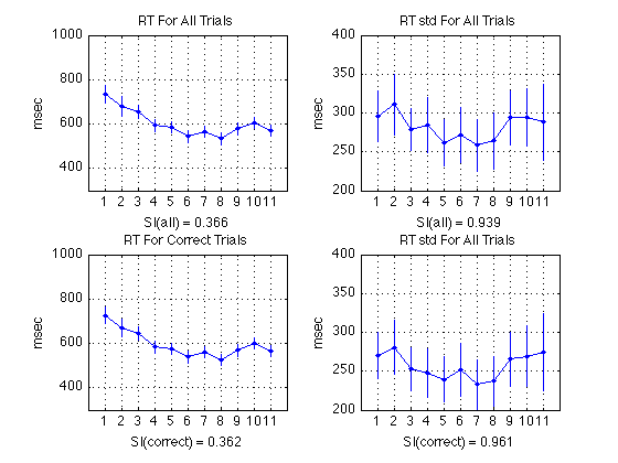
Plot RT and RT std (sbjs averaged together)
% All RTs
subplot(2,2,1) ;
plot(1:N_periods_total, aRT_all, 'b.-') ;
axis([0 N_periods_total+1 300 1000]) ; grid on ;
set(gca,'xtick',([1:N_periods_total]));
title('RT For All Trials') ;
ylabel('msec') ;
xlabel(sprintf('SI(all) = %0.3f', SI_RT_all));
errorbar1(1:N_periods_total,aRT_all,CI_RT_all,['b' 'n']) ;

% Correct RTs
subplot(2,2,3) ;
plot(1:N_periods_total, aRT_corr, 'b.-') ;
axis([0 N_periods_total+1 300 1000]) ; grid on ;
set(gca,'xtick',([1:N_periods_total]));
title('RT For Correct Trials') ;
ylabel('msec') ;
xlabel(sprintf('SI(correct) = %0.3f', SI_RT_corr));
errorbar1(1:N_periods_total,aRT_corr,CI_RT_corr,['b' 'n']) ;

% All RT std
subplot(2,2,2) ;
plot(1:N_periods_total, aRTsd_all, 'b.-') ;
axis([0 N_periods_total+1 200 400]) ; grid on ;
set(gca,'xtick',([1:N_periods_total]));
title('RT std For All Trials') ;
ylabel('msec') ;
xlabel(sprintf('SI(all) = %0.3f', SI_RTsd_all));
errorbar1(1:N_periods_total,aRTsd_all,CI_RTsd_all,['b' 'n']) ;

% Correct RT std
subplot(2,2,4) ;
plot(1:N_periods_total, aRTsd_corr, 'b.-') ;
axis([0 N_periods_total+1 200 400]) ; grid on ;
set(gca,'xtick',([1:N_periods_total]));
title('RT std For All Trials') ;
ylabel('msec') ;
xlabel(sprintf('SI(correct) = %0.3f', SI_RTsd_corr));
errorbar1(1:N_periods_total,aRTsd_corr,CI_RTsd_corr,['b' 'n']) ;
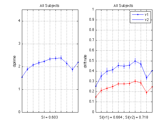
Plot dprime
CI = CI_madpr ;

subplot(1,2,1) ;
plot(1:N_periods_total, mdp11,'b.-') ;
axis([1 N_periods_total 0 M]) ; grid on ;
set(gca,'xtick',([1:N_periods_total]),...
    'xticklabel',[],'ytick',(0:ceil(M))) ;
title('All Subjects') ;
ylabel('dprime');
xlabel(sprintf('SI = %0.3f', SI_dpr));
errorbar1(1:N_periods_total,mdp11,CI,['b' 'n']) ;

% Plot drift rates
subplot(1,2,2) ;
plot(1:N_periods_total, mean(sbj_means(:,v1)), 'b.-');
CI = CI_v1 ;
errorbar1(1:N_periods_total, mean(sbj_means(:,v1)), CI, ['b' 'n']);
hold on
plot(1:N_periods_total, mean(sbj_means(:,v2)), 'r.-');
CI = CI_v2 ;
errorbar1(1:N_periods_total, mean(sbj_means(:,v2)), CI, ['r' 'n']);
axis([1 N_periods_total 0 1]) ; grid on ;
set(gca,'xtick',([1:N_periods_total]),...
    'xticklabel',[],'ytick',(0:.1:1)) ;
title('All Subjects') ;
ylabel('drift rate');
xlabel(sprintf('SI(v1) = %0.3f ; SI(v2) = %0.3f', SI_v1, SI_v2));
legend('v1','v2','location','NorthEast');
hold off
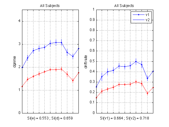
All subjects plot with separate deltas
Delta is easy=7 degrees versus difficult=4 degrees difference b/n clockwise and counterclockwise stimuli.
% Plot dprime
subplot(1,2,1) ;
plot(1:N_periods_total, medp11,'b.-') ;
CI = CI_medpr ;
errorbar1(1:N_periods_total,medp11,CI,['b' 'n']) ;
hold on
plot(1:N_periods_total, mhdp11,'r.-') ;
CI = CI_mhdpr ;
errorbar1(1:N_periods_total,mhdp11,CI,['r' 'n']) ;
axis([1 N_periods_total 0 M]) ; grid on ;
set(gca,'xtick',([1:N_periods_total]),...
    'xticklabel',[],'ytick',(0:ceil(M))) ;
title('All Subjects') ;
ylabel('dprime');
xlabel(sprintf('SI(e) = %0.3f ; SI(d) = %0.3f', SI_edpr, SI_hdpr));

% Plot drift rates
subplot(1,2,2) ;
plot(1:N_periods_total, mean(sbj_means(:,v1)), 'b.-');
CI = CI_v1 ;
errorbar1(1:N_periods_total, mean(sbj_means(:,v1)), CI, ['b' 'n']);
hold on
plot(1:N_periods_total, mean(sbj_means(:,v2)), 'r.-');
CI = CI_v2 ;
errorbar1(1:N_periods_total, mean(sbj_means(:,v2)), CI, ['r' 'n']);
axis([1 N_periods_total 0 1]) ; grid on ;
set(gca,'xtick',([1:N_periods_total]),...
    'xticklabel',[],'ytick',(0:.1:1)) ;
title('All Subjects') ;
ylabel('drift rate');
xlabel(sprintf('SI(v1) = %0.3f ; SI(v2) = %0.3f', SI_v1, SI_v2));
legend('v1','v2','location','NorthEast');
hold off
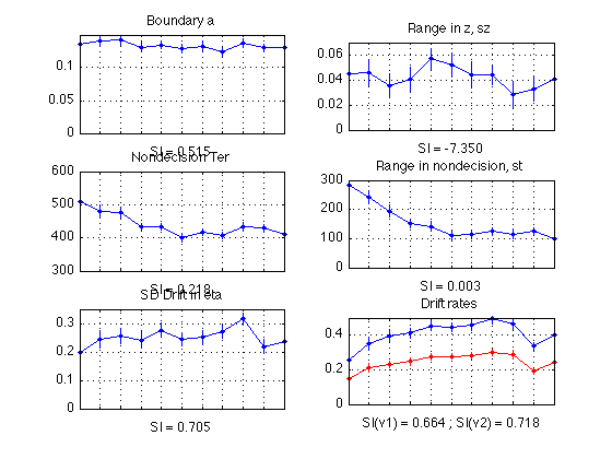
Plot diffusion params (averaged across all sbjs)
MODEL_1, non-bootstrapped, updated for 11 periods, as of 2010-10-21
subplot(3,2,1) ;
% a
plot(1:N_periods_total, mean(sbj_means(:, a)), 'b.-');
CI = CI_a ;
errorbar1(1:N_periods_total, mean(sbj_means(:,a)), CI, ['b' 'n']);
title('Boundary a');
xlabel(sprintf('SI = %0.3f', mean(SI_a)));
set(gca,'xtick',([1:N_periods_total]),'xticklabel',[]);
axis([1 N_periods_total 0 0.15]) ; grid on ;
subplot(3,2,3) ;
% ter
plot(1:N_periods_total, mean(sbj_means(:, ter)*1000), 'b.-');
CI = CI_ter ;
errorbar1(1:N_periods_total, mean(sbj_means(:,ter)*1000), CI*1000, ['b' 'n']);
title('Nondecision Ter');
xlabel(sprintf('SI = %0.3f', mean(SI_ter)));
set(gca,'xtick',([1:N_periods_total]),'xticklabel',[]);
axis([1 N_periods_total 300 600]) ; grid on ;
subplot(3,2,5) ;
% eta
plot(1:N_periods_total, mean(sbj_means(:, eta)), 'b.-');
CI = CI_eta ;
errorbar1(1:N_periods_total, mean(sbj_means(:,eta)), CI, ['b' 'n']);
title('SD Drift in eta');
xlabel(sprintf('SI = %0.3f', mean(SI_eta)));
set(gca,'xtick',([1:N_periods_total]),'xticklabel',[]);
axis([1 N_periods_total 0 0.35]) ; grid on ;
subplot(3,2,2) ;
% sz
plot(1:N_periods_total, mean(sbj_means(:, sz)), 'b.-');
CI = CI_sz ;
errorbar1(1:N_periods_total, mean(sbj_means(:,sz)), CI, ['b' 'n']);
title('Range in z, sz');
xlabel(sprintf('SI = %0.3f', mean(SI_sz)));
set(gca,'xtick',([1:N_periods_total]),'xticklabel',[]);
axis([1 N_periods_total 0 0.07]) ; grid on ;
subplot(3,2,4) ;
% st
plot(1:N_periods_total, mean(sbj_means(:, st)*1000), 'b.-');
CI = CI_st ;
errorbar1(1:N_periods_total, mean(sbj_means(:,st)*1000), CI*1000, ['b' 'n']);
title('Range in nondecision, st');
xlabel(sprintf('SI = %0.3f', mean(SI_st)));
set(gca,'xtick',([1:N_periods_total]),'xticklabel',[]);
axis([1 N_periods_total 0 300]) ; grid on ;
% v1
subplot(3,2,6) ;
plot(1:N_periods_total, mean(sbj_means(:, v1)), 'b.-');
CI = CI_v1 ;
errorbar1(1:N_periods_total, mean(sbj_means(:,v1)), CI, ['b' 'n']);
title('Drift rates');
xlabel(sprintf('SI(v1) = %0.3f ; SI(v2) = %0.3f', mean(SI_v1),mean(SI_v2)));
set(gca,'xtick',([1:N_periods_total]),'xticklabel',[]);
hold on
% v2
plot(1:N_periods_total, mean(sbj_means(:, v2)), 'r.-');
CI = CI_v2 ;
errorbar1(1:N_periods_total, mean(sbj_means(:,v2)), CI, ['r' 'n']);
axis([1 N_periods_total 0 0.5]) ; grid on ;
hold off
Export data for the six-plot empirical figure, 2010-11-17
These data were ported to R and used to generate the main data figure
for the revised manuscript sent to PB&R in November 2010.
They are the group-averaged parameters for the saturated model (MODEL_1)
across the 11 time periods.
% Panel A
fprintf('\n\nEasy dprime: Group mean: medp11 = mean(edp11,2)\n') ;
fprintf(' %6.4f',medp11) ;
fprintf('\n   CI90 w/in sbj:  CI_medpr\n') ;
fprintf(' %6.4f',CI_medpr) ;

fprintf('\n\nHard dprime: Group mean: medp11 = mean(hdp11,2)\n') ;
fprintf(' %6.4f',mhdp11) ;
fprintf('\n   CI90 w/in sbj:  CI_mhdpr\n') ;
fprintf(' %6.4f',CI_mhdpr) ;

fprintf('\n\nAverage dprime (not plotted): Group mean: mdp11 = mean(dp11,2)\n') ;
fprintf(' %6.4f',mdp11) ;
fprintf('\n   CI90 w/in sbj:  CI_madpr\n') ;
fprintf(' %6.4f',CI_madpr) ;


% Panel B
fprintf('\n\nAverage mean RT (all trials): Group mean: aRT_all = mean(sRT_all,1)\n') ;
fprintf(' %6.1f',aRT_all) ;
fprintf('\n   CI90 w/in sbj:  CI_RT_all\n') ;
fprintf(' %6.2f',CI_RT_all) ;


% Panel C
fprintf('\n\nEasy drift rate v1:   mean(sbj_means(:, v1))\n') ;
fprintf(' %6.4f',mean(sbj_means(:, v1))) ;
fprintf('\n   CI90 w/in sbj:  CI_v1\n') ;
fprintf(' %6.4f',CI_v1) ;

fprintf('\n\nHard drift rate v2:   mean(sbj_means(:, v2))\n') ;
fprintf(' %6.4f',mean(sbj_means(:, v2))) ;
fprintf('\n   CI90 w/in sbj:  CI_v2\n') ;
fprintf(' %6.4f',CI_v2) ;


% Panel D
fprintf('\n\nMean nondecision time Ter:   mean(sbj_means(:, ter)*1000)\n') ;
fprintf(' %6.1f',mean(sbj_means(:, ter)*1000)) ;
fprintf('\n   CI90 w/in sbj:  CI_ter*1000\n') ;
fprintf(' %6.2f',CI_ter*1000) ;

fprintf('\n\nRange in nondecision time st (not plotted):   mean(sbj_means(:, st)*1000)\n') ;
fprintf(' %6.1f',mean(sbj_means(:, st)*1000)) ;
fprintf('\n   CI90 w/in sbj:  CI_st*1000\n') ;
fprintf(' %6.2f',CI_st*1000) ;

fprintf('\n\nMinimum nondecision time Tmin=t1:   mean(Tmin,2)*1000\n') ;
fprintf(' %6.1f',mean(Tmin,2)*1000) ;
fprintf('\n   CI90 w/in sbj:  CI_Tmin*1000\n') ;
fprintf(' %6.2f',CI_Tmin*1000) ;


% Panel E
fprintf('\n\nVariability in drift rate eta:   mean(sbj_means(:, eta))\n') ;
fprintf(' %6.4f',mean(sbj_means(:, eta))) ;
fprintf('\n   CI90 w/in sbj:  CI_eta\n') ;
fprintf(' %6.4f',CI_eta) ;


% Panel F
fprintf('\n\nBoundary separation a:   mean(sbj_means(:, a))\n') ;
fprintf(' %6.4f',mean(sbj_means(:, a))) ;
fprintf('\n   CI90 w/in sbj:  CI_a\n') ;
fprintf(' %6.4f',CI_a) ;


% Not plotted
fprintf('\n\nRange in starting point sz:   mean(sbj_means(:, sz))\n') ;
fprintf(' %6.4f',mean(sbj_means(:, sz))) ;
fprintf('\n   CI90 w/in sbj:  CI_sz\n') ;
fprintf(' %6.4f',CI_sz) ;

fprintf('\n\nMAESpec_diffusion_fits executed on %s.\n\n',datestr(now)) ;
Easy dprime: Group mean: medp11 = mean(edp11,2)
 1.9742 2.4024 2.7152 2.8128 2.8620 3.0312 3.0682 3.0706 2.6388 2.4638 2.8112
   CI90 w/in sbj:  CI_medpr
 0.0946 0.1233 0.1219 0.1256 0.0949 0.1272 0.1314 0.1287 0.1476 0.1076 0.1409

Hard dprime: Group mean: medp11 = mean(hdp11,2)
 1.1553 1.4729 1.5972 1.7069 1.7923 1.8890 1.8887 1.9091 1.6944 1.4125 1.7599
   CI90 w/in sbj:  CI_mhdpr
 0.0773 0.0821 0.0729 0.0946 0.0602 0.0731 0.0846 0.0912 0.1305 0.0957 0.0868

Average dprime (not plotted): Group mean: mdp11 = mean(dp11,2)
 1.5379 1.8925 2.0733 2.1644 2.2251 2.3292 2.3588 2.3805 2.1424 1.8721 2.1925
   CI90 w/in sbj:  CI_madpr
 0.0746 0.0791 0.0674 0.0969 0.0577 0.0688 0.0854 0.0966 0.1029 0.0914 0.0901

Average mean RT (all trials): Group mean: aRT_all = mean(sRT_all,1)
  734.2  679.7  655.1  594.0  583.7  543.3  566.7  533.5  579.3  607.0  571.9
   CI90 w/in sbj:  CI_RT_all
  39.64  42.95  29.79  28.62  24.68  25.85  25.90  26.11  26.81  25.60  24.72

Easy drift rate v1:   mean(sbj_means(:, v1))
 0.2541 0.3517 0.3980 0.4133 0.4546 0.4477 0.4588 0.4973 0.4682 0.3358 0.4050
   CI90 w/in sbj:  CI_v1
 0.0280 0.0391 0.0337 0.0297 0.0267 0.0252 0.0336 0.0305 0.0332 0.0244 0.0312

Hard drift rate v2:   mean(sbj_means(:, v2))
 0.1477 0.2118 0.2311 0.2497 0.2776 0.2769 0.2798 0.3023 0.2855 0.1913 0.2461
   CI90 w/in sbj:  CI_v2
 0.0184 0.0243 0.0199 0.0221 0.0192 0.0145 0.0188 0.0204 0.0251 0.0166 0.0191

Mean nondecision time Ter:   mean(sbj_means(:, ter)*1000)
  510.0  479.9  477.6  433.8  433.4  400.6  416.4  406.0  433.3  428.6  409.0
   CI90 w/in sbj:  CI_ter*1000
  26.19  21.09  16.37   9.19   8.98  12.81  10.30   9.44  12.85  10.84  13.18

Range in nondecision time st (not plotted):   mean(sbj_means(:, st)*1000)
  282.7  241.6  194.6  151.1  141.6  110.7  115.8  124.9  115.6  125.4   99.6
   CI90 w/in sbj:  CI_st*1000
  28.45  22.91  21.61  15.39  17.78  13.87  12.67  13.26  16.76  11.55  16.41

Minimum nondecision time Tmin=t1:   mean(Tmin,2)*1000
  368.6  359.1  380.3  358.2  362.6  345.3  358.5  343.5  375.5  365.9  359.2
   CI90 w/in sbj:  CI_Tmin*1000
  35.95  19.85  17.48   8.03   8.92  12.27  10.11   9.68  16.22  10.18  13.63

Variability in drift rate eta:   mean(sbj_means(:, eta))
 0.1974 0.2446 0.2556 0.2412 0.2765 0.2433 0.2500 0.2707 0.3159 0.2191 0.2370
   CI90 w/in sbj:  CI_eta
 0.0314 0.0298 0.0265 0.0295 0.0251 0.0240 0.0254 0.0226 0.0214 0.0268 0.0303

Boundary separation a:   mean(sbj_means(:, a))
 0.1361 0.1415 0.1418 0.1316 0.1346 0.1292 0.1331 0.1238 0.1380 0.1301 0.1311
   CI90 w/in sbj:  CI_a
 0.0099 0.0084 0.0068 0.0069 0.0056 0.0067 0.0069 0.0064 0.0065 0.0053 0.0062

Range in starting point sz:   mean(sbj_means(:, sz))
 0.0454 0.0458 0.0353 0.0407 0.0570 0.0521 0.0440 0.0440 0.0284 0.0331 0.0411
   CI90 w/in sbj:  CI_sz
 0.0105 0.0106 0.0097 0.0094 0.0084 0.0092 0.0106 0.0074 0.0104 0.0102 0.0091

MAESpec_diffusion_fits executed on 29-Nov-2010 17:38:51.
Raw specificity values
'Raw' in the sense that no bootstrapping is involved. Each row printed below represents a subject. Columns are: 1 = dprime 2 = a 3 = Ter 4 = eta 5 = sz 6 = st 7 = v1 8 = v2
% The following indices are calculated
% As of Oct 2010, this code has not been changed since Aug 2010:
%
% SI:   Indices with session 4 used as the final day of training and the
%       first half of session 5 used as the first day of transfer (minus
%       the first block)
% SIb:  Indices with session 5, block 1 used as the final day of training
%       and the first half of session 5 used as the first day of transfer
%       (minus the first block)
% SIc:  Indices with session 4, used as the final day of training and the
%       first block of session 5 used as the first day of "transfer"
%       (although this is not the transfer direction, but a continuation of
%       the training direction occurring after a session of MAE trials)
SI %#ok<*NOPTS>
SIb
SIc
SI =

   -0.2607    1.3000    0.0802    1.8889    0.5181   -0.4750    0.6696    0.5161
    0.6547    0.9167    0.1774    1.6522   -0.2778    0.2548    1.1331    0.9415
    0.7298   -0.9167         0    1.2553   -0.1034   -0.1894    0.4228    1.2258
    0.2035    0.7711    1.7727    0.9346       Inf   -0.1444    0.8756    0.8333
    0.4970   -0.6444    0.1138         0    0.9615    0.0767    0.4468    0.3745
    0.8770   -1.2222    0.0857    2.2973   -1.2000   -0.1172    0.9319    1.1188
    0.6892    0.0328    1.6500    0.6055         0    0.1038    0.6734    0.7415
   -0.1177   -0.1364    0.1327         0         0   -0.0844   -0.0605   -0.0778
    0.9452   -3.8000    0.9577    1.0065      -Inf    0.8957    2.0185    0.6988
    0.4311    0.2297    0.1311       NaN   -0.1452    0.1517    0.1897    0.4954
    0.6626   -0.2500   -0.1923       Inf    1.0000    0.2038    1.0489    0.8302
    1.6666    0.6714    0.2077    0.4136   -0.7778    9.5000    0.8798    1.0328
    0.5775    0.3750    0.4225    4.0714    0.5098   -0.0171    0.2868    0.5665
   -0.2710    0.7838    2.8000    0.5263    0.7619   -0.0776    0.2710    0.4237
    1.3976    0.1667   -0.0441    0.4884    0.1800    0.0144    0.7870    0.8058
    0.1808    0.3731    0.2256    0.2727         0   -0.0636    0.5357    0.3448
    0.8652         0    0.1839   -0.1895   -0.0388   -0.1286    0.6509    0.6864
    1.2435    0.4694   -0.0945       Inf    0.6500    0.0916    1.0652    1.0762
    0.2290    0.2000    0.0412   -1.6885    1.0000    0.1333    2.4921    2.5306
   -0.7018   -1.4615         0  -15.6429    4.9286   -0.7632    2.2975    3.8750
    0.5956   -5.0000    0.2840   28.6667   -4.0000    0.3663    1.1471    1.2000
    0.0224    0.1892    0.0940    0.3533   -1.5172   -0.3412    0.4365    0.3806
    1.3661   -1.2800    0.7101         0   -0.5893   -0.0247    0.2194    0.6243
    0.6933   -0.1389    0.8462    0.5948         0    0.2233    0.8877    0.8919
    0.5132    1.5455    0.1111   -0.1825   -1.6667    0.1024    0.3266    0.4081
    0.5948    0.5536    0.0264    1.0556   -2.7222   -0.2554   -1.4634    0.3514
    2.3037   -1.9444    0.1211   -1.0063    8.8750    0.1453   -0.3471   -1.1000


SIb =

   -0.5717    0.9062   -0.1814    1.1622    0.6226   -1.0345    0.8348    0.7345
    0.8224    1.0159   -0.0200    1.5310   -0.0147   -0.0473    1.1277    0.9588
    0.6772   -0.3529   -0.1429   -3.0000      -Inf   -0.4439    0.4538   -0.4000
    0.2808    0.6984    0.7792    0.9296    2.9143    0.2961    0.9051    0.7222
   -0.9064    0.0263    0.0763         0      -Inf    0.2136   -0.1094   -0.2836
    0.7626   -0.2903    0.4921    2.2973    0.7027   -0.2361    0.8932    1.1739
    0.5443   -0.9667    0.0250    0.7471    6.0000    0.0717    0.6957    0.7551
   -0.1602   -2.1250   -6.7273         0         0    0.3949   -0.0273   -0.0112
    0.8829    0.7000    0.9423    1.0274   -9.3333    0.7536    1.9016    1.2907
   -0.5315   -0.3902    0.1264       NaN      -Inf    0.0682    0.1856   -0.8644
    0.5400    3.5000   -4.1667    0.8688    1.0000    0.5098    1.5625    3.2500
   -6.1749    0.2813    0.2426    0.4974      -Inf   -2.0357    0.8372    1.5714
    0.4931    0.1818    0.0682    0.6417    0.7396    0.0556    0.2581    0.6364
   -1.5157    0.4286   -1.5714    0.7300    0.9123    0.1935    0.2427    0.0377
    1.4272    0.5000   -0.1639    0.4907   -0.2424   -0.2018    0.8145    0.8050
   -0.1316    0.4545    0.2536    0.0345         0    0.2812   -0.0777   -0.0857
    0.3192    0.2667    0.1839         0         0    0.1124    0.2377    0.2697
    2.2789   -1.1667   -0.1583    1.0283    0.8923    0.0165    1.0898    1.0597
    0.1014    6.0000   -1.1136   -4.4667       NaN    0.2778    2.6207   -1.0270
   -0.4198   -3.5714    0.0780   -0.3314         0   -1.7917   -0.1716   -0.5753
    0.5772   -0.2414    0.3980    2.2029    2.0526    0.1351    1.0820    1.1532
    0.5466   -0.8182   -0.0495    0.6151   -1.4333   -0.0560    0.6606    0.6706
    1.1675   -0.1176    1.5714         0   -0.7800   -0.0473    0.4158    0.7948
    0.3447   -0.2424    2.5000    0.6737         0   -0.0335    0.8834    0.8660
    0.2741    0.4545    0.2000         0    1.4000    0.3294    0.0163   -0.0126
    0.6248    0.3902   -0.4832    0.9747   -0.1552   -0.2419   -0.0100    0.8812
    1.2691    8.5714    0.0044       Inf    3.8636   -0.2645   -1.8596    1.6364


SIc =

    0.1979    4.2000    0.2214   -4.4815   -0.2771    0.2750   -1.0000   -0.8226
   -0.9441    6.2500    0.1935   -0.2283   -0.2593    0.2885   -0.0418   -0.4211
    0.1631   -0.4167    0.1250    1.0638    1.0000    0.1762   -0.0569    1.1613
   -0.1074    0.2410    4.5000    0.0719      -Inf   -0.6257   -0.3111    0.4000
    0.7362   -0.6889    0.0407         0    1.0000   -0.1742    0.5013    0.5127
    0.4819   -0.7222   -0.8000         0   -6.4000    0.0962    0.3624    0.3168
    0.3181    0.5082    1.6667   -0.5596    1.2000    0.0346   -0.0730   -0.0554
    0.0367    0.6364    0.8878         0         0   -0.7922   -0.0323   -0.0659
    0.5319  -15.0000    0.2676    0.7630      -Inf    0.5767   -0.1296    2.0361
    0.6285    0.4459    0.0055       NaN    1.0000    0.0897    0.0051    0.7294
    0.2664    1.5000    0.7692       Inf    0.0345   -0.6242    0.9130    1.0755
    1.0929    0.5429   -0.0462   -0.1667    1.0000    3.8000    0.2618    0.9426
    0.1665    0.2361    0.3803    9.5714   -0.8824   -0.0769    0.0388   -0.1921
    0.4948    0.6216    1.7000   -0.7544   -1.7143   -0.3362    0.0374    0.4011
    0.0695   -0.6667    0.1029   -0.0047    0.3400    0.1799   -0.1480    0.0041
    0.2760   -0.1493   -0.0376    0.2468         0   -0.4798    0.5692    0.3966
    0.8020   -0.3636         0   -0.1895   -0.0388   -0.2714    0.5421    0.5706
    0.8096    0.7551    0.0551      -Inf   -2.2500    0.0763    0.2739   -0.2762
    0.1421    1.1600    0.5464    0.5082    1.0000   -0.2000    0.0794    1.7551
   -0.1986    0.4615   -0.0847  -11.5000    4.9286    0.3684    2.1074    2.8250
    0.0434   -3.8333   -0.1893  -22.0000    5.7500    0.2673   -0.7941   -0.3053
   -1.1563    0.5541    0.1368   -0.6800   -0.0345   -0.2701   -0.6599   -0.8806
   -1.1858   -1.0400    1.5072         0    0.1071    0.0216   -0.3361   -0.8307
    0.5321    0.0833    1.1026   -0.2416         0    0.2484    0.0367    0.1931
    0.3294    2.0000   -0.1111   -0.1825    7.6667   -0.3386    0.3154    0.4154
   -0.0798    0.2679    0.3436    3.1944   -2.2222   -0.0109   -1.4390   -4.4595
   -3.8451    1.3889    0.1172    1.0000   -1.7500    0.3240    0.5289    4.3000
Diffusion paramter specificity values (avg across subjs)
SI_a
SI_ter
SI_eta
SI_sz
SI_st
SI_v1
SI_v2
SI_a =

    0.5150


SI_ter =

    0.2175


SI_eta =

    0.7048


SI_sz =

   -7.3500


SI_st =

    0.0031


SI_v1 =

    0.6641


SI_v2 =

    0.7181
Bootstrap Specificity Indices and Confidence Intervals
N_samples = 1000 ;

% If the bootstrapping has already been run, just load the file B.mat
% Delete this file to rerun the bootstrap process...
filename = fullfile(MAESpec02_pathstr,'diffusion','B.mat') ;
%recalculatep = true ;
recalculatep = false ;
if (recalculatep || ~exist(filename,'file'))

    for k = N_samples:-1:1    % work backwards so that B(1000) is allocated first
        %- Sample subjects with replacement within each group
        if (k==1)  % very fist sample always is the full data set
            sample = sbj_means ;
			% The new diffusion models
			sample2 = df_2 ;
			sample3 = df_3 ;
			sample4 = df_4 ;
            RT_all_sample = sRT_all ;
            RT_corr_sample = sRT_corr ;
            RTsd_all_sample = RTsd_all ;
            RTsd_corr_sample = RTsd_corr ;
        else
            idx = ceil(rand(1,N_sbj).*N_sbj) ;
			% Separate randomization for each model (is this necessary?)
			idx2 = ceil(rand(1,N_sbj).*N_sbj) ;
			idx3 = ceil(rand(1,N_sbj).*N_sbj) ;
			idx4 = ceil(rand(1,N_sbj).*N_sbj) ;
            sample = sbj_means(idx,:) ;
			sample2 = df_2(idx2,:) ;
			sample3 = df_3(idx3,:) ;
			sample4 = df_4(idx4,:) ;
            RT_all_sample = sRT_all(idx,:) ;
            RT_corr_sample = sRT_corr(idx,:) ;
            RTsd_all_sample = RTsd_all(idx,:) ;
            RTsd_corr_sample = RTsd_corr(idx,:) ;
        end

        % Pack this data away for later use
        % This is MODEL_1, which existed (without a subscript) prior to
        % October 2010.  The indices were updated 2010-10-20 to accommodate
        % that now there are 11 periods instead of 8.  Otherwise it's the
        % same.
        B(k).adpr = sample(:,dpr) ;
        B(k).edpr = sample(:,edpr_idx) ;
        B(k).hdpr = sample(:,hdpr_idx) ;
        B(k).a = sample(:,a) ;
        B(k).ter = sample(:,ter) ;
        B(k).eta = sample(:,eta) ;
        B(k).sz = sample(:,sz) ;
        B(k).st = sample(:,st) ;
        B(k).v1 = sample(:,v1) ;
        B(k).v2 = sample(:,v2) ;
        B(k).v_avg = (sample(:,v1) + sample(:,v2)) ./ 2 ;
        B(k).t1 = sample(:,ter) - (sample(:,st) ./ 2);
        B(k).t2 = sample(:,ter) + (sample(:,st) ./ 2);
        B(k).RT_all = RT_all_sample ;
        B(k).RT_corr = RT_corr_sample ;
        B(k).RTsd_all = RTsd_all_sample ;
        B(k).RTsd_corr = RTsd_corr_sample ;

		% Pack away the NEW diffusion model params (3 new models)
		% MODEL_2 -- added 2010-10-20 using MODEL_1 as a template
		B(k).a_2 = sample2(:,a_2) ;
		B(k).ter_2 = sample2(:,ter_2) ;
		B(k).eta_2 = sample2(:,eta_2) ;
        B(k).sz_2 = sample2(:,sz_2) ;
		B(k).st_2 = sample2(:,st_2) ;
		B(k).v1_2 = sample2(:,v1_2) ;
		B(k).v2_2 = sample2(:,v2_2) ;
		B(k).v_avg_2 = (sample2(:,v1_2) + sample2(:,v2_2)) ./ 2 ;
		B(k).t1_2 = sample2(:,ter_2) - (sample2(:,st_2) ./ 2);
        B(k).t2_2 = sample2(:,ter_2) + (sample2(:,st_2) ./ 2);

		% MODEL_3 -- added 2010-10-20 using MODEL_1 as a template
		B(k).a_3 = sample3(:,a_3) ;
		B(k).ter_3 = sample3(:,ter_3) ;
		B(k).eta_3 = sample3(:,eta_3) ;
        B(k).sz_3 = sample3(:,sz_3) ;
		B(k).st_3 = sample3(:,st_3) ;
		B(k).v1_3 = sample3(:,v1_3) ;
		B(k).v2_3 = sample3(:,v2_3) ;
		B(k).v_avg_3 = (sample3(:,v1_3) + sample3(:,v2_3)) ./ 2 ;
		B(k).t1_3 = sample3(:,ter_3) - repmat((sample3(:,st_3)./2),1,N_periods_total);
        B(k).t2_3 = sample3(:,ter_3) + repmat((sample3(:,st_3)./2),1,N_periods_total);

		% MODEL_4 -- added 2010-10-20 using MODEL_1 as a template
		B(k).a_4 = sample4(:,a_4) ;
		B(k).ter_4 = sample4(:,ter_4) ;
		B(k).eta_4 = sample4(:,eta_4) ;
        B(k).sz_4 = sample4(:,sz_4) ;
		B(k).st_4 = sample4(:,st_4) ;
		B(k).v1_4 = sample4(:,v1_4) ;
		B(k).v2_4 = sample4(:,v2_4) ;
		B(k).v_avg_4 = (sample4(:,v1_4) + sample4(:,v2_4)) ./ 2 ;
		B(k).t1_4 = sample4(:,ter_4) - (sample4(:,st_4) ./ 2);
        B(k).t2_4 = sample4(:,ter_4) + (sample4(:,st_4) ./ 2);

        % Pack away the specificity values for each
        smean = mean(sample,1) ;
		smean2 = mean(sample2,1) ;
        smean3 = mean(sample3,1) ;
		smean4 = mean(sample4,1) ;

        %tmp = smean(dpr) ;    % obsolete code, subsumed within @specif_idx
        %B(k).adpr_SI = (tmp(5) - tmp(7))/ (tmp(5) - tmp(1)) ;
        B(k).adpr_SI = specif_idx(smean(dpr)) ;
        B(k).edpr_SI = specif_idx(smean(edpr_idx)) ;
        B(k).hdpr_SI = specif_idx(smean(hdpr_idx)) ;
        B(k).a_SI = specif_idx(smean(a)) ;
        B(k).ter_SI = specif_idx(smean(ter)) ;
        B(k).eta_SI = specif_idx(smean(eta)) ;
        B(k).sz_SI = specif_idx(smean(sz)) ;
        B(k).st_SI = specif_idx(smean(st)) ;
        B(k).v1_SI = specif_idx(smean(v1)) ;
        B(k).v2_SI = specif_idx(smean(v2)) ;
        B(k).v_avg_SI = specif_idx(mean(B(k).v_avg,1)) ;
        % the 'gain' is drift relative to dprime
        B(k).gain_SI = B(k).v_avg_SI - B(k).adpr_SI ;
        B(k).t1_SI = specif_idx(mean(B(k).t1,1)) ;
        B(k).t2_SI = specif_idx(mean(B(k).t2,1)) ;
        B(k).RT_all_SI = specif_idx(mean(B(k).RT_all,1)) ;
        B(k).RT_corr_SI = specif_idx(mean(B(k).RT_corr,1)) ;
        B(k).RTsd_all_SI = specif_idx(mean(B(k).RTsd_all,1)) ;
        B(k).RTsd_corr_SI = specif_idx(mean(B(k).RTsd_corr,1)) ;

        % The 3 new diffusion models. The fields that are fixed across all
        % periods for a particular model are commented out because no
        % specificity index can be calculated for them. 2010-10-21

		% Model 2 -- this is the most constrainted model. Only drift rates
		% vary across periods, so there is only SI for drift
		%B(k).a_SI_2 = specif_idx(smean2(a_2)) ;
        %B(k).ter_SI_2 = specif_idx(smean2(ter_2)) ;
        %B(k).eta_SI_2 = specif_idx(smean2(eta_2)) ;
        %B(k).sz_SI_2 = specif_idx(smean2(sz_2)) ;
        %B(k).st_SI_2 = specif_idx(smean2(st_2)) ;
        B(k).v1_SI_2 = specif_idx(smean2(v1_2)) ;
        B(k).v2_SI_2 = specif_idx(smean2(v2_2)) ;
        B(k).v_avg_SI_2 = specif_idx(mean(B(k).v_avg_2,1)) ;
        B(k).gain_SI_2 = B(k).v_avg_SI_2 - B(k).adpr_SI ;
        %B(k).t1_SI_2 = specif_idx(mean(B(k).t1_2,1)) ;
        %B(k).t2_SI_2 = specif_idx(mean(B(k).t2_2,1)) ;

		% Model 3 -- Ter and drift vary and hence have SIs
		%B(k).a_SI_3 = specif_idx(smean3(a_3)) ;
        B(k).ter_SI_3 = specif_idx(smean3(ter_3)) ;
        %B(k).eta_SI_3 = specif_idx(smean3(eta_3)) ;
        %B(k).sz_SI_3 = specif_idx(smean3(sz_3)) ;
        %B(k).st_SI_3 = specif_idx(smean3(st_3)) ;
        B(k).v1_SI_3 = specif_idx(smean3(v1_3)) ;
        B(k).v2_SI_3 = specif_idx(smean3(v2_3)) ;
        B(k).v_avg_SI_3 = specif_idx(mean(B(k).v_avg_3,1)) ;
        B(k).gain_SI_3 = B(k).v_avg_SI_3 - B(k).adpr_SI ;
        %B(k).t1_SI_3 = specif_idx(mean(B(k).t1_3,1)) ;
        %B(k).t2_SI_3 = specif_idx(mean(B(k).t2_3,1)) ;

		% Model 4 -- Ter, st, and drift vary. Eta, a, and sz are fixed.
		%B(k).a_SI_4 = specif_idx(smean4(a_4)) ;
        B(k).ter_SI_4 = specif_idx(smean4(ter_4)) ;
        %B(k).eta_SI_4 = specif_idx(smean4(eta_4)) ;
        %B(k).sz_SI_4 = specif_idx(smean4(sz_4)) ;
        B(k).st_SI_4 = specif_idx(smean4(st_4)) ;
        B(k).v1_SI_4 = specif_idx(smean4(v1_4)) ;
        B(k).v2_SI_4 = specif_idx(smean4(v2_4)) ;
        B(k).v_avg_SI_4 = specif_idx(mean(B(k).v_avg_4,1)) ;
        B(k).gain_SI_4 = B(k).v_avg_SI_4 - B(k).adpr_SI ;
        B(k).t1_SI_4 = specif_idx(mean(B(k).t1_4,1)) ;
        B(k).t2_SI_4 = specif_idx(mean(B(k).t2_4,1)) ;

        % Learning indices *********************************************
        B(k).adpr_LI = learn_idx(smean(dpr)) ;
        B(k).edpr_LI = learn_idx(smean(edpr_idx)) ;
        B(k).hdpr_LI = learn_idx(smean(hdpr_idx)) ;
        B(k).a_LI = learn_idx(smean(a)) ;
        B(k).ter_LI = learn_idx(smean(ter)) ;
        B(k).eta_LI = learn_idx(smean(eta)) ;
        B(k).sz_LI = learn_idx(smean(sz)) ;
        B(k).st_LI = learn_idx(smean(st)) ;
        B(k).v1_LI = learn_idx(smean(v1)) ;
        B(k).v2_LI = learn_idx(smean(v2)) ;
        B(k).v_avg_LI = learn_idx(mean(B(k).v_avg,1)) ;
        B(k).gain_LI = B(k).v_avg_LI - B(k).adpr_LI ;
        B(k).t1_LI = learn_idx(mean(B(k).t1,1)) ;
        B(k).t2_LI = learn_idx(mean(B(k).t2,1)) ;
        B(k).RT_all_LI = learn_idx(mean(B(k).RT_all,1)) ;
        B(k).RT_corr_LI = learn_idx(mean(B(k).RT_corr,1)) ;
        B(k).RTsd_all_LI = learn_idx(mean(B(k).RTsd_all,1)) ;
        B(k).RTsd_corr_LI = learn_idx(mean(B(k).RTsd_corr,1)) ;

        % The 3 new diffusion models. The fields that are fixed across all
        % periods for a particular model are commented out because no
        % learning index can be calculated for them. 2010-10-21

		% Model 2 -- this is the most constrainted model. Only drift rates
		% vary across periods, so there is only LI for drift
		%B(k).a_LI_2 = learn_idx(smean2(a_2)) ;
        %B(k).ter_LI_2 = learn_idx(smean2(ter_2)) ;
        %B(k).eta_LI_2 = learn_idx(smean2(eta_2)) ;
        %B(k).sz_LI_2 = learn_idx(smean2(sz_2)) ;
        %B(k).st_LI_2 = learn_idx(smean2(st_2)) ;
        B(k).v1_LI_2 = learn_idx(smean2(v1_2)) ;
        B(k).v2_LI_2 = learn_idx(smean2(v2_2)) ;
        B(k).v_avg_LI_2 = learn_idx(mean(B(k).v_avg_2,1)) ;
        B(k).gain_LI_2 = B(k).v_avg_LI_2 - B(k).adpr_LI ;
        %B(k).t1_LI_2 = learn_idx(mean(B(k).t1_2,1)) ;
        %B(k).t2_LI_2 = learn_idx(mean(B(k).t2_2,1)) ;

        % Model 3 -- Ter and drift vary and hence have LIs
		%B(k).a_LI_3 = learn_idx(smean3(a_3)) ;
        B(k).ter_LI_3 = learn_idx(smean3(ter_3)) ;
        %B(k).eta_LI_3 = learn_idx(smean3(eta_3)) ;
        %B(k).sz_LI_3 = learn_idx(smean3(sz_3)) ;
        %B(k).st_LI_3 = learn_idx(smean3(st_3)) ;
        B(k).v1_LI_3 = learn_idx(smean3(v1_3)) ;
        B(k).v2_LI_3 = learn_idx(smean3(v2_3)) ;
        B(k).v_avg_LI_3 = learn_idx(mean(B(k).v_avg_3,1)) ;
        B(k).gain_LI_3 = B(k).v_avg_LI_3 - B(k).adpr_LI ;
        %B(k).t1_LI_3 = learn_idx(mean(B(k).t1_3,1)) ;
        %B(k).t2_LI_3 = learn_idx(mean(B(k).t2_3,1)) ;

        % Model 4 -- Ter, st, and drift vary. Eta, a, and sz are fixed.
		%B(k).a_LI_4 = learn_idx(smean4(a_4)) ;
        B(k).ter_LI_4 = learn_idx(smean4(ter_4)) ;
        %B(k).eta_LI_4 = learn_idx(smean4(eta_4)) ;
        %B(k).sz_LI_4 = learn_idx(smean4(sz_4)) ;
        B(k).st_LI_4 = learn_idx(smean4(st_4)) ;
        B(k).v1_LI_4 = learn_idx(smean4(v1_4)) ;
        B(k).v2_LI_4 = learn_idx(smean4(v2_4)) ;
        B(k).v_avg_LI_4 = learn_idx(mean(B(k).v_avg_4,1)) ;
        B(k).gain_LI_4 = B(k).v_avg_LI_4 - B(k).adpr_LI ;
        B(k).t1_LI_4 = learn_idx(mean(B(k).t1_4,1)) ;
        B(k).t2_LI_4 = learn_idx(mean(B(k).t2_4,1)) ;

    end
    clear tmp;

    % Save the structure B for later
    save(filename,'B') ;
else
    fprintf('load %s \n\n',filename) ;
    load(filename) ;
end
load /Users/apetrov/a/r/w/work/MLExper/MAESpec02/diffusion/B.mat
B(1) contains the SIs and LIs on the full data set
B(1)
ans =

            adpr: [27x11 double]
            edpr: [27x11 double]
            hdpr: [27x11 double]
               a: [27x11 double]
             ter: [27x11 double]
             eta: [27x11 double]
              sz: [27x11 double]
              st: [27x11 double]
              v1: [27x11 double]
              v2: [27x11 double]
           v_avg: [27x11 double]
              t1: [27x11 double]
              t2: [27x11 double]
          RT_all: [27x11 double]
         RT_corr: [27x11 double]
        RTsd_all: [27x11 double]
       RTsd_corr: [27x11 double]
             a_2: [27x1 double]
           ter_2: [27x1 double]
           eta_2: [27x1 double]
            sz_2: [27x1 double]
            st_2: [27x1 double]
            v1_2: [27x11 double]
            v2_2: [27x11 double]
         v_avg_2: [27x11 double]
            t1_2: [27x1 double]
            t2_2: [27x1 double]
             a_3: [27x1 double]
           ter_3: [27x11 double]
           eta_3: [27x1 double]
            sz_3: [27x1 double]
            st_3: [27x1 double]
            v1_3: [27x11 double]
            v2_3: [27x11 double]
         v_avg_3: [27x11 double]
            t1_3: [27x11 double]
            t2_3: [27x11 double]
             a_4: [27x1 double]
           ter_4: [27x11 double]
           eta_4: [27x1 double]
            sz_4: [27x1 double]
            st_4: [27x11 double]
            v1_4: [27x11 double]
            v2_4: [27x11 double]
         v_avg_4: [27x11 double]
            t1_4: [27x11 double]
            t2_4: [27x11 double]
         adpr_SI: 0.6034
         edpr_SI: 0.5534
         hdpr_SI: 0.6588
            a_SI: 0.5150
          ter_SI: 0.2175
          eta_SI: 0.7048
           sz_SI: -7.3500
           st_SI: 0.0031
           v1_SI: 0.6641
           v2_SI: 0.7181
        v_avg_SI: 0.6851
         gain_SI: 0.0816
           t1_SI: 0.8909
           t2_SI: 0.1250
       RT_all_SI: 0.3660
      RT_corr_SI: 0.3621
     RTsd_all_SI: 0.9392
    RTsd_corr_SI: 0.9614
         v1_SI_2: 0.6230
         v2_SI_2: 0.6793
      v_avg_SI_2: 0.6427
       gain_SI_2: 0.0393
        ter_SI_3: 0.3880
         v1_SI_3: 0.5503
         v2_SI_3: 0.6685
      v_avg_SI_3: 0.5950
       gain_SI_3: -0.0085
        ter_SI_4: 0.3174
         st_SI_4: 0.2316
         v1_SI_4: 0.5642
         v2_SI_4: 0.6636
      v_avg_SI_4: 0.6029
       gain_SI_4: -5.3980e-04
         t1_SI_4: 0.4890
         t2_SI_4: 0.2831
         adpr_LI: 0.5478
         edpr_LI: 0.5554
         hdpr_LI: 0.6525
            a_LI: -0.0909
          ter_LI: -0.2040
          eta_LI: 0.3710
           sz_LI: -0.0326
           st_LI: -0.5582
           v1_LI: 0.9573
           v2_LI: 1.0469
        v_avg_LI: 0.9902
         gain_LI: 0.4424
           t1_LI: -0.0682
           t2_LI: -0.2809
       RT_all_LI: -0.2734
      RT_corr_LI: -0.2734
     RTsd_all_LI: -0.1072
    RTsd_corr_LI: -0.1236
         v1_LI_2: 1.0282
         v2_LI_2: 0.9050
      v_avg_LI_2: 0.9814
       gain_LI_2: 0.4336
        ter_LI_3: -0.2040
         v1_LI_3: 0.7731
         v2_LI_3: 0.7936
      v_avg_LI_3: 0.7807
       gain_LI_3: 0.2329
        ter_LI_4: -0.2588
         st_LI_4: -0.6169
         v1_LI_4: 0.6760
         v2_LI_4: 0.7411
      v_avg_LI_4: 0.6999
       gain_LI_4: 0.1521
         t1_LI_4: -0.1198
         t2_LI_4: -0.3370
Average over all N_samples to find more stable SI values
MODEL_1, which prior to Oct 2010 was the only model -- the saturated model
SI_adpr_b = [B.adpr_SI]' ;
SI_edpr_b = [B.edpr_SI]' ;
SI_hdpr_b = [B.hdpr_SI]' ;
SI_a_b = [B.a_SI]' ;
SI_ter_b = [B.ter_SI]' ;
SI_eta_b = [B.eta_SI]' ;
SI_sz_b = [B.sz_SI]' ;
SI_st_b = [B.st_SI]' ;
SI_v1_b = [B.v1_SI]' ;
SI_v2_b = [B.v2_SI]' ;
% The three new models (2 thourgh 4), as of 2010-10-20:
SI_v1_b_2 = [B.v1_SI_2]' ;
SI_v2_b_2 = [B.v2_SI_2]' ;
SI_v1_b_3 = [B.v1_SI_3]' ;
SI_v2_b_3 = [B.v2_SI_3]' ;
SI_ter_b_3 = [B.ter_SI_3]' ;
SI_v1_b_4 = [B.v1_SI_4]' ;
SI_v2_b_4 = [B.v2_SI_4]' ;
SI_ter_b_4 = [B.ter_SI_4]' ;
SI_st_b_4 = [B.st_SI_4]' ;
% Special averaged drift rate
SI_v_avg_b = [B.v_avg_SI]' ;
SI_v_avg_b_2 = [B.v_avg_SI_2]' ;
SI_v_avg_b_3 = [B.v_avg_SI_3]' ;
SI_v_avg_b_4 = [B.v_avg_SI_4]' ;
% Special "gain" over traditional dprime analysis
SI_gain_b = [B.gain_SI]' ;
SI_gain_b_2 = [B.gain_SI_2]' ;
SI_gain_b_3 = [B.gain_SI_3]' ;
SI_gain_b_4 = [B.gain_SI_4]' ;
% Define Ter/St interaction variables
SI_t1_b = [B.t1_SI]' ;
SI_t2_b = [B.t2_SI]' ;
SI_t1_b_4 = [B.t1_SI_4]' ;
SI_t2_b_4 = [B.t2_SI_4]' ;
SI_RT_all_b = [B.RT_all_SI]' ;
SI_RT_corr_b = [B.RT_corr_SI]' ;
SI_RTsd_all_b = [B.RTsd_all_SI]' ;
SI_RTsd_corr_b = [B.RTsd_corr_SI]' ;
Average over all N_samples to find more stable LI values
MODEL_1, which prior to Oct 2010 was the only model -- the saturated model
LI_adpr_b = [B.adpr_LI]' ;
LI_edpr_b = [B.edpr_LI]' ;
LI_hdpr_b = [B.hdpr_LI]' ;
LI_a_b = [B.a_LI]' ;
LI_ter_b = [B.ter_LI]' ;
LI_eta_b = [B.eta_LI]' ;
LI_sz_b = [B.sz_LI]' ;
LI_st_b = [B.st_LI]' ;
LI_v1_b = [B.v1_LI]' ;
LI_v2_b = [B.v2_LI]' ;
% The three new models (2 thourgh 4), as of 2010-10-20:
LI_v1_b_2 = [B.v1_LI_2]' ;
LI_v2_b_2 = [B.v2_LI_2]' ;
LI_v1_b_3 = [B.v1_LI_3]' ;
LI_v2_b_3 = [B.v2_LI_3]' ;
LI_ter_b_3 = [B.ter_LI_3]' ;
LI_v1_b_4 = [B.v1_LI_4]' ;
LI_v2_b_4 = [B.v2_LI_4]' ;
LI_ter_b_4 = [B.ter_LI_4]' ;
LI_st_b_4 = [B.st_LI_4]' ;

% Special averaged drift rate
LI_v_avg_b = [B.v_avg_LI]' ;
LI_v_avg_b_2 = [B.v_avg_LI_2]' ;
LI_v_avg_b_3 = [B.v_avg_LI_3]' ;
LI_v_avg_b_4 = [B.v_avg_LI_4]' ;
% Special "gain" over traditional dprime analysis
LI_gain_b = [B.gain_LI]' ;
LI_gain_b_2 = [B.gain_LI_2]' ;
LI_gain_b_3 = [B.gain_LI_3]' ;
LI_gain_b_4 = [B.gain_LI_4]' ;
% Define Ter/St interaction variables
LI_t1_b = [B.t1_LI]' ;
LI_t2_b = [B.t2_LI]' ;
LI_t1_b_4 = [B.t1_LI_4]' ;
LI_t2_b_4 = [B.t2_LI_4]' ;
LI_RT_all_b = [B.RT_all_LI]' ;
LI_RT_corr_b = [B.RT_corr_LI]' ;
LI_RTsd_all_b = [B.RTsd_all_LI]' ;
LI_RTsd_corr_b = [B.RTsd_corr_LI]' ;
Collect distribution statistics of the 11-point profiles
D-prime
adpr_gr = NaN(N_samples, N_periods_total) ;
edpr_gr = NaN(N_samples, N_periods_total) ;
hdpr_gr = NaN(N_samples, N_periods_total) ;

% MODEL_1
a_gr = NaN(N_samples, N_periods_total) ;
ter_gr = NaN(N_samples, N_periods_total) ;
eta_gr = NaN(N_samples, N_periods_total) ;
sz_gr = NaN(N_samples, N_periods_total) ;
st_gr = NaN(N_samples, N_periods_total) ;
v1_gr = NaN(N_samples, N_periods_total) ;
v2_gr = NaN(N_samples, N_periods_total) ;
% Special averaged drift rate
v_avg_gr = NaN(N_samples,N_periods_total) ;
t1_gr = NaN(N_samples,N_periods_total) ;
t2_gr = NaN(N_samples,N_periods_total) ;
RT_all_gr = NaN(N_samples,N_periods_total) ;
RT_corr_gr = NaN(N_samples,N_periods_total) ;
RTsd_all_gr = NaN(N_samples,N_periods_total) ;
RTsd_corr_gr = NaN(N_samples,N_periods_total) ;

% The three new models (featuring 11-point profiles)
% Model 2:
a_gr_2 = NaN(N_samples, 1) ;
ter_gr_2 = NaN(N_samples, 1) ;
eta_gr_2 = NaN(N_samples, 1) ;
sz_gr_2 = NaN(N_samples, 1) ;
st_gr_2 = NaN(N_samples, 1) ;
v1_gr_2 = NaN(N_samples, N_periods_total) ;
v2_gr_2 = NaN(N_samples, N_periods_total) ;
% Special averaged drift rate
v_avg_gr_2 = NaN(N_samples,N_periods_total) ;

% Model 3:
a_gr_3 = NaN(N_samples, 1) ;
eta_gr_3 = NaN(N_samples, 1) ;
sz_gr_3 = NaN(N_samples, 1) ;
st_gr_3 = NaN(N_samples, 1) ;
ter_gr_3 = NaN(N_samples, N_periods_total) ;
v1_gr_3 = NaN(N_samples, N_periods_total) ;
v2_gr_3 = NaN(N_samples, N_periods_total) ;
% Special averaged drift rate
v_avg_gr_3 = NaN(N_samples,N_periods_total) ;

% Model 4:
a_gr_4 = NaN(N_samples, 1) ;
eta_gr_4 = NaN(N_samples, 1) ;
sz_gr_4 = NaN(N_samples, 1) ;
ter_gr_4 = NaN(N_samples, N_periods_total) ;
st_gr_4 = NaN(N_samples, N_periods_total) ;
v1_gr_4 = NaN(N_samples, N_periods_total) ;
v2_gr_4 = NaN(N_samples, N_periods_total) ;
% Special averaged drift rate
v_avg_gr_4 = NaN(N_samples,N_periods_total) ;


% Calculate averages across the bootstrap samples
for k=1:N_samples
    % Eleven-point curves for each group
    % D-prime
    adpr_gr(k,:) = mean(B(k).adpr,1) ;
    edpr_gr(k,:) = mean(B(k).edpr,1) ;
    hdpr_gr(k,:) = mean(B(k).hdpr,1) ;

    % Model 1
    a_gr(k,:) = mean(B(k).a,1) ;
    ter_gr(k,:) = mean(B(k).ter,1) ;
    eta_gr(k,:) = mean(B(k).eta,1) ;
    sz_gr(k,:) = mean(B(k).sz,1) ;
    st_gr(k,:) = mean(B(k).st,1) ;
    v1_gr(k,:) = mean(B(k).v1,1) ;
    v2_gr(k,:) = mean(B(k).v2,1) ;
    v_avg_gr(k,:) = mean(B(k).v_avg,1) ;
    t1_gr(k,:) = mean(B(k).t1,1) ;
    t2_gr(k,:) = mean(B(k).t2,1) ;
    RT_all_gr(k,:) = mean(B(k).RT_all,1) ;
    RT_corr_gr(k,:) = mean(B(k).RT_corr,1) ;
    RTsd_all_gr(k,:) = mean(B(k).RTsd_all,1) ;
    RTsd_corr_gr(k,:) = mean(B(k).RTsd_corr,1) ;

	% The three new models
	% Model 2
	a_gr_2(k,:) = mean(B(k).a_2,1) ;
    ter_gr_2(k,:) = mean(B(k).ter_2,1) ;
    eta_gr_2(k,:) = mean(B(k).eta_2,1) ;
    sz_gr_2(k,:) = mean(B(k).sz_2,1) ;
    st_gr_2(k,:) = mean(B(k).st_2,1) ;
	v1_gr_2(k,:) = mean(B(k).v1_2,1) ;
    v2_gr_2(k,:) = mean(B(k).v2_2,1) ;
    v_avg_gr_2(k,:) = mean(B(k).v_avg_2,1) ;

	% Model 3
	a_gr_3(k,:) = mean(B(k).a_3,1) ;
    eta_gr_3(k,:) = mean(B(k).eta_3,1) ;
    sz_gr_3(k,:) = mean(B(k).sz_3,1) ;
    st_gr_3(k,:) = mean(B(k).st_3,1) ;
	ter_gr_3(k,:) = mean(B(k).ter_3,1) ;
	v1_gr_3(k,:) = mean(B(k).v1_3,1) ;
    v2_gr_3(k,:) = mean(B(k).v2_3,1) ;
    v_avg_gr_3(k,:) = mean(B(k).v_avg_3,1) ;

	% Model 4
	a_gr_4(k,:) = mean(B(k).a_4,1) ;
    eta_gr_4(k,:) = mean(B(k).eta_4,1) ;
    sz_gr_4(k,:) = mean(B(k).sz_4,1) ;
	ter_gr_4(k,:) = mean(B(k).ter_4,1) ;
	st_gr_4(k,:) = mean(B(k).st_4,1) ;
	v1_gr_4(k,:) = mean(B(k).v1_4,1) ;
    v2_gr_4(k,:) = mean(B(k).v2_4,1) ;
    v_avg_gr_4(k,:) = mean(B(k).v_avg_4,1) ;
end
Plot bootstrap dprime curve and SI value for single dprime
This is old code (prior to 2010-10-21) -- the aggregate-dprime version of panel a in Figure~2.
% Find BS confidence interval
bs_adpr = prctile(adpr_gr,[10 50 90],1) ;

figure
% Single dprime curve
M = 3.5 ;
plot(1:N_periods_total, bs_adpr(2,:),'b.-') ;
axis([1 N_periods_total 0 M]) ; grid on ;
set(gca,'xtick',([1:N_periods_total]),...
    'xticklabel',[],'ytick',(0:ceil(M))) ;
title(sprintf('Bootstrap dprime for %d samples', N_samples)) ;
ylabel('dprime');
xlabel(sprintf('SI = %0.3f', (median(SI_adpr_b))));
errorbar1(1:N_periods_total,bs_adpr(2,:),bs_adpr(2,:) - bs_adpr(1,:),...
    bs_adpr(3,:) - bs_adpr(2,:)) ;
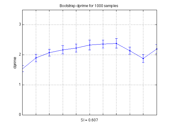
Bootstrap-based dprime learning curves
Plot bootstrap dprime curves and SI values for easy and hard dprime Panel A in Figure 2 in the PBR manuscript submitted 2010-08-03. Updated to 11 time periods 2010-10-21 NOTE: This was abandoned in the revision of 2010-11-17. The revised figure does not use any bootstrap values. It is based on the empirical means and the within-subject CIs instead -- see the above section titled "Export data for the six-plot empirical figure, 2010-11-17".
% Find BS confidence interval
bs_edpr = prctile(edpr_gr,[10 50 90],1) ;
bs_hdpr = prctile(hdpr_gr,[10 50 90],1) ;

figure
% Easy and difficult dprimes
plot(1:N_periods_total, bs_edpr(2,:),'b.-') ;
errorbar1(1:N_periods_total,bs_edpr(2,:),bs_edpr(2,:) - bs_edpr(1,:),...
    bs_edpr(3,:) - bs_edpr(2,:),'b') ;
hold on
plot(1:N_periods_total, bs_hdpr(2,:),'r.-') ;
errorbar1(1:N_periods_total,bs_hdpr(2,:),bs_hdpr(2,:) - bs_hdpr(1,:),...
    bs_hdpr(3,:) - bs_hdpr(2,:), 'r') ;
axis([1 N_periods_total 0 M]) ; grid on ;
set(gca,'xtick',([1:N_periods_total]),...
    'xticklabel',[],'ytick',(0:ceil(M))) ;
title(sprintf('Bootstrap dprime for %d samples', N_samples)) ;
ylabel('dprime');
xlabel(sprintf('SI(e) = %0.3f ; SI(d) = %0.3f', median(SI_edpr_b), median(SI_hdpr_b)));
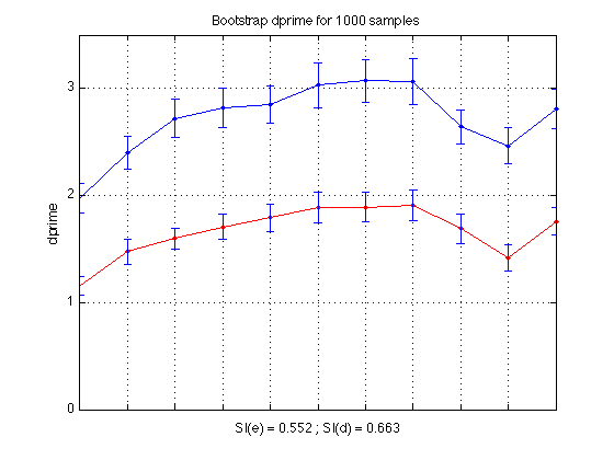
Plot the resulting diffusion param bootstrap curves with SI written below
Old (prior to Oct 2010) ==> All for the saturated MODEL 1. Updated for 11 periods, 2010-10-21.
% Find BS confidence interval
bs_a = prctile(a_gr,[10 50 90],1) ;
bs_ter = prctile(ter_gr,[10 50 90],1) ;
bs_eta = prctile(eta_gr,[10 50 90],1) ;
bs_sz = prctile(sz_gr,[10 50 90],1) ;
bs_st = prctile(st_gr,[10 50 90],1) ;
bs_v1 = prctile(v1_gr,[10 50 90],1) ;
bs_v2 = prctile(v2_gr,[10 50 90],1) ;
bs_v_avg = prctile(v_avg_gr,[10 50 90],1) ;

figure
subplot(3,2,1) ;
% a
plot(1:N_periods_total, bs_a(2,:), 'b.-');
errorbar1(1:N_periods_total,bs_a(2,:),bs_a(2,:) - bs_a(1,:),...
    bs_a(3,:) - bs_a(2,:)) ;
title('Boundary a');
xlabel(sprintf('SI = %0.3f', median(SI_a_b)));
set(gca,'xtick',([1:N_periods_total]),'xticklabel',[]);
axis([1 N_periods_total 0.10 0.15]) ; grid on ;
subplot(3,2,3) ;
% ter
plot(1:N_periods_total, bs_ter(2,:)*1000, 'b.-');
errorbar1(1:N_periods_total,bs_ter(2,:)*1000,(bs_ter(2,:) - bs_ter(1,:))*1000,...
    (bs_ter(3,:) - bs_ter(2,:))*1000) ;
title('Nondecision Ter');
xlabel(sprintf('SI = %0.3f', median(SI_ter_b)));
set(gca,'xtick',([1:N_periods_total]),'xticklabel',[]);
axis([1 N_periods_total 300 600]) ; grid on ;
subplot(3,2,5) ;
% eta
plot(1:N_periods_total, bs_eta(2,:), 'b.-');
errorbar1(1:N_periods_total,bs_eta(2,:),bs_eta(2,:) - bs_eta(1,:),...
    bs_eta(3,:) - bs_eta(2,:)) ;
title('SD Drift in eta');
xlabel(sprintf('SI = %0.3f', median(SI_eta_b)));
set(gca,'xtick',([1:N_periods_total]),'xticklabel',[]);
axis([1 N_periods_total 0 0.35]) ; grid on ;
subplot(3,2,2) ;
% sz
plot(1:N_periods_total, bs_sz(2,:), 'b.-');
errorbar1(1:N_periods_total,bs_sz(2,:),bs_sz(2,:) - bs_sz(1,:),...
    bs_sz(3,:) - bs_sz(2,:)) ;
title('Range in z, sz');
xlabel(sprintf('SI = %0.3f', median(SI_sz_b)));
set(gca,'xtick',([1:N_periods_total]),'xticklabel',[]);
axis([1 N_periods_total 0 0.07]) ; grid on ;
subplot(3,2,4) ;
% st
plot(1:N_periods_total, bs_st(2,:)*1000, 'b.-');
errorbar1(1:N_periods_total,bs_st(2,:)*1000,(bs_st(2,:) - bs_st(1,:))*1000,...
    (bs_st(3,:) - bs_st(2,:))*1000) ;
title('Range in nondecision, st');
xlabel(sprintf('SI = %0.3f', median(SI_st_b)));
set(gca,'xtick',([1:N_periods_total]),'xticklabel',[]);
axis([1 N_periods_total 0 300]) ; grid on ;
% v1
subplot(3,2,6) ;
plot(1:N_periods_total, bs_v1(2,:), 'b.-');
errorbar1(1:N_periods_total,bs_v1(2,:),bs_v1(2,:) - bs_v1(1,:),...
    bs_v1(3,:) - bs_v1(2,:)) ;
title('Drift rates');
xlabel(sprintf('SI(v1) = %0.3f ; v = %0.3f ; SI(v2) = %0.3f',...
    median(SI_v1_b),median(SI_v_avg_b),median(SI_v2_b)));
set(gca,'xtick',([1:N_periods_total]),'xticklabel',[]);
hold on
% v2
plot(1:N_periods_total, bs_v2(2,:), 'r.-');
errorbar1(1:N_periods_total,bs_v2(2,:),bs_v2(2,:) - bs_v2(1,:),...
    bs_v2(3,:) - bs_v2(2,:)) ;
axis([1 N_periods_total 0 0.5]) ; grid on ;
% v avg
hold on
plot(1:N_periods_total, bs_v_avg(2,:), 'g.-');
errorbar1(1:N_periods_total,bs_v_avg(2,:),bs_v_avg(2,:) - bs_v_avg(1,:),...
    bs_v_avg(3,:) - bs_v_avg(2,:)) ;
hold off
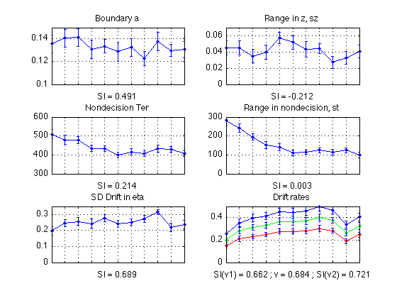
Ter analysis
Old (prior to Oct 2010) ==> All for the saturated MODEL 1. Updated for 11 periods, 2010-10-21.
bs_t1 = prctile(t1_gr,[10 50 90],1) ;
bs_t2 = prctile(t2_gr,[10 50 90],1) ;

figure
subplot(2,2,1) ;
% ter
plot(1:N_periods_total, bs_ter(2,:)*1000, 'b.-');
errorbar1(1:N_periods_total,bs_ter(2,:)*1000,(bs_ter(2,:) - bs_ter(1,:))*1000,...
    (bs_ter(3,:) - bs_ter(2,:))*1000) ;
title('Nondecision Ter');
xlabel(sprintf('SI = %0.3f', median(SI_ter_b)));
set(gca,'xtick',([1:N_periods_total]),'xticklabel',[]);
axis([1 N_periods_total 300 600]) ; grid on ;
subplot(2,2,2) ;
% st
plot(1:N_periods_total, bs_st(2,:)*1000, 'b.-');
errorbar1(1:N_periods_total,bs_st(2,:)*1000,(bs_st(2,:) - bs_st(1,:))*1000,...
    (bs_st(3,:) - bs_st(2,:))*1000) ;
title('Range in nondecision, st');
xlabel(sprintf('SI = %0.3f', median(SI_st_b)));
set(gca,'xtick',([1:N_periods_total]),'xticklabel',[]);
axis([1 N_periods_total 0 300]) ; grid on ;
subplot(2,2,3) ;
% Ter - st/2 = t1
plot(1:N_periods_total, bs_t1(2,:)*1000, 'b.-');
errorbar1(1:N_periods_total,bs_t1(2,:)*1000,(bs_t1(2,:) - bs_t1(1,:))*1000,...
    (bs_t1(3,:) - bs_t1(2,:))*1000) ;
title('Minimum non-decision time t1');
xlabel(sprintf('SI = %0.3f', median(SI_t1_b)));
set(gca,'xtick',([1:N_periods_total]),'xticklabel',[]);
axis([1 N_periods_total 300 600]) ; grid on ;
subplot(2,2,4) ;
% Ter + st/2 = t2
plot(1:N_periods_total, bs_t2(2,:)*1000, 'b.-');
errorbar1(1:N_periods_total,bs_t2(2,:)*1000,(bs_t2(2,:) - bs_t2(1,:))*1000,...
    (bs_t2(3,:) - bs_t2(2,:))*1000) ;
title('Maximum non--decision time t2');
xlabel(sprintf('SI = %0.3f', median(SI_t2_b)));
set(gca,'xtick',([1:N_periods_total]),'xticklabel',[]);
axis([1 N_periods_total 400 700]) ; grid on ;
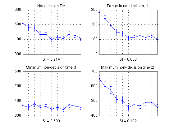
New diffusion models (2-4)
This code was added by Nick 2010-10-20
% Find BS confidence interval
% Model 2
bs_a_2 = prctile(a_gr_2,[10 50 90],1) ;
bs_ter_2 = prctile(ter_gr_2,[10 50 90],1) ;
bs_eta_2 = prctile(eta_gr_2,[10 50 90],1) ;
bs_sz_2 = prctile(sz_gr_2,[10 50 90],1) ;
bs_st_2 = prctile(st_gr_2,[10 50 90],1) ;
bs_v1_2 = prctile(v1_gr_2,[10 50 90],1) ;
bs_v2_2 = prctile(v2_gr_2,[10 50 90],1) ;
bs_v_avg_2 = prctile(v_avg_gr_2,[10 50 90],1) ;

% Model 3
bs_a_3 = prctile(a_gr_3,[10 50 90],1) ;
bs_ter_3 = prctile(ter_gr_3,[10 50 90],1) ;
bs_eta_3 = prctile(eta_gr_3,[10 50 90],1) ;
bs_sz_3 = prctile(sz_gr_3,[10 50 90],1) ;
bs_st_3 = prctile(st_gr_3,[10 50 90],1) ;
bs_v1_3 = prctile(v1_gr_3,[10 50 90],1) ;
bs_v2_3 = prctile(v2_gr_3,[10 50 90],1) ;
bs_v_avg_3 = prctile(v_avg_gr_3,[10 50 90],1) ;

% Model 4
bs_a_4 = prctile(a_gr_4,[10 50 90],1) ;
bs_ter_4 = prctile(ter_gr_4,[10 50 90],1) ;
bs_eta_4 = prctile(eta_gr_4,[10 50 90],1) ;
bs_sz_4 = prctile(sz_gr_4,[10 50 90],1) ;
bs_st_4 = prctile(st_gr_4,[10 50 90],1) ;
bs_v1_4 = prctile(v1_gr_4,[10 50 90],1) ;
bs_v2_4 = prctile(v2_gr_4,[10 50 90],1) ;
bs_v_avg_4 = prctile(v_avg_gr_4,[10 50 90],1) ;

figure
% Plot model 2 (only drift rates apply here)
% v1
subplot(3,3,1) ;
plot(1:N_periods_total, bs_v1_2(2,:), 'b.-');
errorbar1(1:N_periods_total,bs_v1_2(2,:),bs_v1_2(2,:) - bs_v1_2(1,:),...
    bs_v1_2(3,:) - bs_v1_2(2,:)) ;
title('Drift rates (Model 2)');
xlabel(sprintf('SI(v1) = %0.3f ; v = %0.3f ; SI(v2) = %0.3f',...
    median(SI_v1_b_2),median(SI_v_avg_b_2),median(SI_v2_b_2)));
set(gca,'xtick',([1:N_periods_total]),'xticklabel',[]);
hold on
% v2
plot(1:N_periods_total, bs_v2_2(2,:), 'r.-');
errorbar1(1:N_periods_total,bs_v2_2(2,:),bs_v2_2(2,:) - bs_v2_2(1,:),...
    bs_v2_2(3,:) - bs_v2_2(2,:)) ;
axis([1 N_periods_total 0 0.5]) ; grid on ;
% v avg
hold on
plot(1:N_periods_total, bs_v_avg_2(2,:), 'g.-');
errorbar1(1:N_periods_total,bs_v_avg_2(2,:),bs_v_avg_2(2,:) - bs_v_avg_2(1,:),...
    bs_v_avg_2(3,:) - bs_v_avg_2(2,:)) ;
hold off

% Plot model 3
% v1
subplot(3,3,4) ;
plot(1:N_periods_total, bs_v1_3(2,:), 'b.-');
errorbar1(1:N_periods_total,bs_v1_3(2,:),bs_v1_3(2,:) - bs_v1_3(1,:),...
    bs_v1_3(3,:) - bs_v1_3(2,:)) ;
title('Drift rates (Model 3)');
xlabel(sprintf('SI(v1) = %0.3f ; v = %0.3f ; SI(v2) = %0.3f',...
    median(SI_v1_b_3),median(SI_v_avg_b_3),median(SI_v2_b_3)));
set(gca,'xtick',([1:N_periods_total]),'xticklabel',[]);
hold on
% v2
plot(1:N_periods_total, bs_v2_3(2,:), 'r.-');
errorbar1(1:N_periods_total,bs_v2_3(2,:),bs_v2_3(2,:) - bs_v2_3(1,:),...
    bs_v2_3(3,:) - bs_v2_3(2,:)) ;
axis([1 N_periods_total 0 0.5]) ; grid on ;
% v avg
hold on
plot(1:N_periods_total, bs_v_avg_3(2,:), 'g.-');
errorbar1(1:N_periods_total,bs_v_avg_3(2,:),bs_v_avg_3(2,:) - bs_v_avg_3(1,:),...
    bs_v_avg_3(3,:) - bs_v_avg_3(2,:)) ;
hold off
% ter
subplot(3,3,5) ;
plot(1:N_periods_total, bs_ter_3(2,:)*1000, 'b.-');
errorbar1(1:N_periods_total,bs_ter_3(2,:)*1000,(bs_ter_3(2,:) - bs_ter_3(1,:))*1000,...
    (bs_ter_3(3,:) - bs_ter_3(2,:))*1000) ;
title('Nondec Ter (Model 3)');
xlabel(sprintf('SI = %0.3f', median(SI_ter_b_3)));
set(gca,'xtick',([1:N_periods_total]),'xticklabel',[]);
axis([1 N_periods_total 300 600]) ; grid on ;

% Plot model 4
subplot(3,3,7) ;
% v1
plot(1:N_periods_total, bs_v1_4(2,:), 'b.-');
errorbar1(1:N_periods_total,bs_v1_4(2,:),bs_v1_4(2,:) - bs_v1_4(1,:),...
    bs_v1_4(3,:) - bs_v1_4(2,:)) ;
title('Drift rates (Model 4)');
xlabel(sprintf('SI(v1) = %0.3f ; v = %0.3f ; SI(v2) = %0.3f',...
    median(SI_v1_b_4),median(SI_v_avg_b_4),median(SI_v2_b_4)));
set(gca,'xtick',([1:N_periods_total]),'xticklabel',[]);
hold on
% v2
plot(1:N_periods_total, bs_v2_4(2,:), 'r.-');
errorbar1(1:N_periods_total,bs_v2_4(2,:),bs_v2_4(2,:) - bs_v2_4(1,:),...
    bs_v2_4(3,:) - bs_v2_4(2,:)) ;
axis([1 N_periods_total 0 0.5]) ; grid on ;
% v avg
hold on
plot(1:N_periods_total, bs_v_avg_4(2,:), 'g.-');
errorbar1(1:N_periods_total,bs_v_avg_4(2,:),bs_v_avg_4(2,:) - bs_v_avg_4(1,:),...
    bs_v_avg_4(3,:) - bs_v_avg_4(2,:)) ;
hold off
% ter
subplot(3,3,8) ;
plot(1:N_periods_total, bs_ter_4(2,:)*1000, 'b.-');
errorbar1(1:N_periods_total,bs_ter_4(2,:)*1000,(bs_ter_4(2,:) - bs_ter_4(1,:))*1000,...
    (bs_ter_4(3,:) - bs_ter_4(2,:))*1000) ;
title('Nondec Ter (Model 4)');
xlabel(sprintf('SI = %0.3f', median(SI_ter_b_4)));
set(gca,'xtick',([1:N_periods_total]),'xticklabel',[]);
axis([1 N_periods_total 300 600]) ; grid on ;
% st
subplot(3,3,9) ;
plot(1:N_periods_total, bs_st_4(2,:)*1000, 'b.-');
errorbar1(1:N_periods_total,bs_st_4(2,:)*1000,(bs_st_4(2,:) - bs_st_4(1,:))*1000,...
    (bs_st_4(3,:) - bs_st_4(2,:))*1000) ;
title('Rng in nondec, st (Model 4)');
xlabel(sprintf('SI = %0.3f', median(SI_st_b_4)));
set(gca,'xtick',([1:N_periods_total]),'xticklabel',[]);
axis([1 N_periods_total 0 300]) ; grid on ;
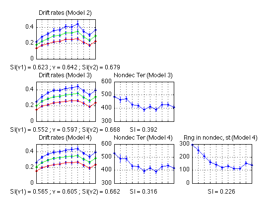
Plot Bootstrap RT and RT std (sbjs averaged together)
Old (prior to Oct 2010). Based on bootstrapping the raw RTs Updated for 11 periods, 2010-10-21.
% Find BS confidence interval
bs_RT_all = prctile(RT_all_gr,[10 50 90],1) ;
bs_RT_corr = prctile(RT_corr_gr,[10 50 90],1) ;
bs_RTsd_all = prctile(RTsd_all_gr,[10 50 90],1) ;
bs_RTsd_corr = prctile(RTsd_corr_gr,[10 50 90],1) ;

% All RTs
subplot(2,2,1) ;
plot(1:N_periods_total, bs_RT_all(2,:), 'b.-') ;
axis([1 N_periods_total 400 800]) ; grid on ;
set(gca,'xtick',([1:N_periods_total]));
title('RT For All Trials') ;
ylabel('msec') ;
xlabel(sprintf('SI = %0.3f', median(SI_RT_all_b)));
errorbar1(1:N_periods_total,bs_RT_all(2,:),bs_RT_all(2,:) - bs_RT_all(1,:),...
    bs_RT_all(3,:) - bs_RT_all(2,:)) ;

% Correct RTs
subplot(2,2,3) ;
plot(1:N_periods_total, bs_RT_corr(2,:), 'b.-') ;
axis([1 N_periods_total 400 800]) ; grid on ;
set(gca,'xtick',([1:N_periods_total]));
title('RT For Correct Trials') ;
ylabel('msec') ;
xlabel(sprintf('SI = %0.3f', median(SI_RT_corr_b)));
errorbar1(1:N_periods_total,bs_RT_corr(2,:),bs_RT_corr(2,:) - bs_RT_corr(1,:),...
    bs_RT_corr(3,:) - bs_RT_corr(2,:)) ;

% All RT std
subplot(2,2,2) ;
plot(1:N_periods_total, bs_RTsd_all(2,:), 'b.-') ;
axis([1 N_periods_total 200 400]) ; grid on ;
set(gca,'xtick',([1:N_periods_total]));
title('RT std For All Trials') ;
ylabel('msec') ;
xlabel(sprintf('SI = %0.3f', median(SI_RTsd_all_b)));
errorbar1(1:N_periods_total,bs_RTsd_all(2,:),bs_RTsd_all(2,:) - bs_RTsd_all(1,:),...
    bs_RTsd_all(3,:) - bs_RTsd_all(2,:)) ;

% Correct RT std
subplot(2,2,4) ;
plot(1:N_periods_total, bs_RTsd_corr(2,:), 'b.-') ;
axis([1 N_periods_total 200 400]) ; grid on ;
set(gca,'xtick',([1:N_periods_total]));
title('RT std For All Trials') ;
ylabel('msec') ;
xlabel(sprintf('SI = %0.3f', median(SI_RTsd_corr_b)));
errorbar1(1:N_periods_total,bs_RTsd_corr(2,:),bs_RTsd_corr(2,:) - bs_RTsd_corr(1,:),...
    bs_RTsd_corr(3,:) - bs_RTsd_corr(2,:)) ;
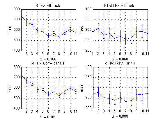
Raw bootstrap percentiles
fprintf('\n---------------------------------------------\n')
fprintf('Raw data statistics\n');
fprintf('---------------------------------------------\n')
fprintf('Row 1 = Lower bound   (10th percentile)\n');
fprintf('Row 2 = Median        (50th percentile)\n');
fprintf('Row 3 = Upper bound   (90th percentile)\n');
fprintf('\nColumns = Eight "blocks"\n');
fprintf('---------------------------------------------\n')
% All dprime
bs_adpr
% Easy dprime
bs_edpr
% Hard dprime
bs_hdpr
% All RTs
bs_RT_all
% Correct RTs
bs_RT_corr
% All RTs std
bs_RTsd_all
% Correct RTs std
bs_RTsd_corr
% Diffusion params
bs_a
bs_ter
bs_eta
bs_sz
bs_st
bs_v1
bs_v2
bs_v_avg
bs_t1
bs_t2
% Diffusion Model 2
bs_a_2
bs_ter_2
bs_eta_2
bs_sz_2
bs_st_2
bs_v1_2
bs_v2_2
bs_v_avg_2
% Diffusion Model 3
bs_a_3
bs_ter_3
bs_eta_3
bs_sz_3
bs_st_3
bs_v1_3
bs_v2_3
bs_v_avg_3
% Diffusion Model 4
bs_a_4
bs_ter_4
bs_eta_4
bs_sz_4
bs_st_4
bs_v1_4
bs_v2_4
bs_v_avg_4
---------------------------------------------
Raw data statistics
---------------------------------------------
Row 1 = Lower bound   (10th percentile)
Row 2 = Median        (50th percentile)
Row 3 = Upper bound   (90th percentile)

Columns = Eight "blocks"
---------------------------------------------

bs_adpr =

    1.4367    1.7657    1.9649    2.0288    2.0930    2.1692    2.2237    2.2244    2.0168    1.7400    2.0548
    1.5393    1.8934    2.0750    2.1690    2.2242    2.3303    2.3597    2.3820    2.1384    1.8744    2.1955
    1.6471    2.0170    2.1983    2.2967    2.3647    2.4955    2.4971    2.5308    2.2709    2.0035    2.3351


bs_edpr =

    1.8416    2.2488    2.5407    2.6314    2.6777    2.8155    2.8753    2.8518    2.4783    2.2962    2.6301
    1.9759    2.4028    2.7216    2.8181    2.8518    3.0297    3.0738    3.0680    2.6409    2.4637    2.8137
    2.1140    2.5631    2.9010    2.9966    3.0467    3.2535    3.2572    3.2808    2.7956    2.6332    2.9891


bs_hdpr =

    1.0725    1.3564    1.4994    1.5867    1.6649    1.7461    1.7577    1.7639    1.5554    1.2910    1.6334
    1.1569    1.4745    1.5988    1.7069    1.7911    1.8907    1.8925    1.9093    1.6917    1.4161    1.7602
    1.2422    1.5894    1.7003    1.8349    1.9276    2.0382    2.0234    2.0503    1.8419    1.5266    1.8968


bs_RT_all =

  702.8218  645.6204  631.5556  571.7940  564.8542  524.1273  546.3194  513.1389  558.1574  587.0741  553.0926
  732.6065  677.7894  654.3472  593.2269  582.7639  541.9398  566.0463  532.2870  578.9444  606.0231  570.7685
  762.6759  711.8171  676.2477  616.0093  601.2917  562.3727  587.5278  553.8032  599.7593  626.0949  591.5154


bs_RT_corr =

  695.2593  636.7037  620.9815  563.0602  558.7292  519.5162  540.0347  507.7153  547.2500  579.5162  548.0556
  723.9306  667.6319  643.8310  583.6319  575.9213  536.9028  559.6991  526.2569  567.9259  598.2755  565.1049
  753.1528  701.1250  664.9120  605.8449  593.9699  557.1806  580.1713  547.1412  588.9722  618.3218  585.8179


bs_RTsd_all =

  271.2380  281.7221  258.8286  256.0314  238.9274  242.1797  234.1187  235.2190  265.0464  263.9384  249.0007
  293.4101  306.9057  276.3318  282.0221  261.0090  269.4625  257.1695  262.6774  292.2507  292.3318  285.2090
  320.2189  340.8848  298.3680  308.6940  282.6419  297.4763  282.2577  288.1292  319.2524  321.1733  323.1568


bs_RTsd_corr =

  248.6649  253.7839  233.0209  222.2371  217.0721  224.7152  209.2572  212.2859  237.1992  237.8397  234.8352
  269.2033  277.5831  250.7157  246.2273  238.3459  250.7240  231.5255  235.5596  264.8405  267.1865  271.7885
  292.2763  306.2322  272.4131  269.4260  259.1715  277.2152  255.8084  258.1075  290.1545  298.2473  311.3206


bs_a =

    0.1278    0.1328    0.1336    0.1229    0.1276    0.1206    0.1249    0.1166    0.1295    0.1247    0.1234
    0.1358    0.1407    0.1414    0.1311    0.1337    0.1288    0.1327    0.1229    0.1376    0.1300    0.1306
    0.1436    0.1495    0.1489    0.1398    0.1415    0.1367    0.1405    0.1306    0.1450    0.1355    0.1379


bs_ter =

    0.4869    0.4555    0.4579    0.4167    0.4169    0.3851    0.3995    0.3900    0.4134    0.4127    0.3925
    0.5098    0.4797    0.4774    0.4340    0.4328    0.4001    0.4155    0.4051    0.4325    0.4279    0.4078
    0.5340    0.5061    0.4970    0.4520    0.4517    0.4184    0.4348    0.4245    0.4538    0.4465    0.4279


bs_eta =

    0.1714    0.2216    0.2334    0.2146    0.2560    0.2213    0.2305    0.2485    0.3013    0.1939    0.2101
    0.1982    0.2456    0.2567    0.2426    0.2767    0.2435    0.2504    0.2712    0.3159    0.2205    0.2372
    0.2245    0.2699    0.2773    0.2684    0.2962    0.2656    0.2685    0.2934    0.3291    0.2449    0.2624


bs_sz =

    0.0360    0.0365    0.0263    0.0311    0.0500    0.0437    0.0339    0.0378    0.0200    0.0252    0.0330
    0.0448    0.0453    0.0350    0.0400    0.0574    0.0518    0.0436    0.0439    0.0274    0.0329    0.0407
    0.0539    0.0549    0.0442    0.0498    0.0637    0.0596    0.0530    0.0500    0.0367    0.0415    0.0482


bs_st =

    0.2587    0.2194    0.1766    0.1314    0.1223    0.0964    0.1036    0.1109    0.1003    0.1119    0.0842
    0.2820    0.2415    0.1937    0.1505    0.1406    0.1104    0.1150    0.1242    0.1151    0.1250    0.0997
    0.3049    0.2637    0.2117    0.1694    0.1598    0.1245    0.1269    0.1383    0.1295    0.1376    0.1142


bs_v1 =

    0.2272    0.3192    0.3670    0.3841    0.4231    0.4146    0.4185    0.4592    0.4355    0.3047    0.3689
    0.2553    0.3539    0.3987    0.4144    0.4543    0.4489    0.4601    0.4989    0.4678    0.3373    0.4059
    0.2845    0.3877    0.4307    0.4463    0.4882    0.4824    0.4975    0.5329    0.4988    0.3704    0.4396


bs_v2 =

    0.1314    0.1886    0.2140    0.2289    0.2553    0.2543    0.2554    0.2771    0.2630    0.1707    0.2234
    0.1480    0.2133    0.2312    0.2501    0.2782    0.2784    0.2808    0.3035    0.2839    0.1926    0.2469
    0.1666    0.2358    0.2500    0.2720    0.3014    0.3017    0.3030    0.3273    0.3091    0.2125    0.2691


bs_v_avg =

    0.1797    0.2547    0.2908    0.3068    0.3391    0.3341    0.3375    0.3684    0.3507    0.2382    0.2968
    0.2015    0.2838    0.3150    0.3321    0.3660    0.3636    0.3705    0.4016    0.3764    0.2647    0.3265
    0.2253    0.3119    0.3401    0.3581    0.3942    0.3910    0.4004    0.4301    0.4021    0.2909    0.3545


bs_t1 =

    0.3409    0.3392    0.3620    0.3453    0.3478    0.3308    0.3435    0.3287    0.3555    0.3515    0.3439
    0.3686    0.3584    0.3805    0.3583    0.3620    0.3446    0.3583    0.3431    0.3748    0.3654    0.3587
    0.3986    0.3812    0.3990    0.3722    0.3791    0.3616    0.3757    0.3602    0.3972    0.3825    0.3761


bs_t2 =

    0.6298    0.5672    0.5503    0.4842    0.4810    0.4362    0.4545    0.4483    0.4683    0.4723    0.4377
    0.6514    0.6006    0.5744    0.5095    0.5038    0.4557    0.4735    0.4676    0.4905    0.4905    0.4576
    0.6731    0.6344    0.5982    0.5341    0.5277    0.4778    0.4946    0.4902    0.5142    0.5114    0.4810


bs_a_2 =

    0.1336
    0.1385
    0.1433


bs_ter_2 =

    0.3928
    0.4076
    0.4269


bs_eta_2 =

    0.1972
    0.2163
    0.2347


bs_sz_2 =

    0.0310
    0.0379
    0.0445


bs_st_2 =

    0.1512
    0.1710
    0.1920


bs_v1_2 =

    0.2013    0.2571    0.2904    0.3395    0.3430    0.3816    0.3735    0.4021    0.3269    0.2825    0.3416
    0.2174    0.2752    0.3127    0.3615    0.3662    0.4082    0.4053    0.4395    0.3490    0.3016    0.3659
    0.2342    0.2940    0.3363    0.3844    0.3910    0.4358    0.4381    0.4829    0.3724    0.3230    0.3882


bs_v2_2 =

    0.1214    0.1571    0.1743    0.2014    0.2071    0.2244    0.2251    0.2332    0.1919    0.1573    0.2044
    0.1331    0.1711    0.1878    0.2164    0.2244    0.2442    0.2444    0.2540    0.2087    0.1717    0.2205
    0.1449    0.1848    0.2016    0.2309    0.2423    0.2629    0.2633    0.2769    0.2284    0.1871    0.2373


bs_v_avg_2 =

    0.1615    0.2077    0.2324    0.2706    0.2752    0.3044    0.2993    0.3181    0.2614    0.2198    0.2744
    0.1753    0.2231    0.2503    0.2891    0.2954    0.3263    0.3252    0.3468    0.2782    0.2367    0.2931
    0.1891    0.2391    0.2680    0.3074    0.3159    0.3489    0.3504    0.3794    0.2987    0.2546    0.3120


bs_a_3 =

    0.1319
    0.1368
    0.1416


bs_ter_3 =

    0.4628    0.4406    0.4506    0.4084    0.4042    0.3744    0.3965    0.3730    0.4059    0.4124    0.3940
    0.4865    0.4627    0.4696    0.4243    0.4193    0.3890    0.4123    0.3877    0.4243    0.4264    0.4075
    0.5124    0.4872    0.4889    0.4426    0.4363    0.4076    0.4302    0.4057    0.4426    0.4439    0.4249


bs_eta_3 =

    0.2194
    0.2374
    0.2556


bs_sz_3 =

    0.0416
    0.0496
    0.0570


bs_st_3 =

    0.1279
    0.1406
    0.1525


bs_v1_3 =

    0.2317    0.2936    0.3402    0.3692    0.3733    0.3917    0.3981    0.4127    0.3608    0.3112    0.3659
    0.2473    0.3124    0.3590    0.3893    0.3917    0.4160    0.4241    0.4386    0.3817    0.3322    0.3898
    0.2626    0.3287    0.3782    0.4095    0.4126    0.4407    0.4523    0.4638    0.4023    0.3556    0.4141


bs_v2_3 =

    0.1379    0.1760    0.1990    0.2196    0.2243    0.2384    0.2423    0.2447    0.2116    0.1701    0.2183
    0.1466    0.1900    0.2099    0.2350    0.2390    0.2553    0.2591    0.2624    0.2292    0.1848    0.2332
    0.1549    0.2037    0.2210    0.2506    0.2553    0.2736    0.2760    0.2799    0.2481    0.2000    0.2475


bs_v_avg_3 =

    0.1852    0.2360    0.2701    0.2947    0.2994    0.3167    0.3204    0.3297    0.2892    0.2407    0.2926
    0.1969    0.2511    0.2843    0.3120    0.3153    0.3353    0.3416    0.3502    0.3049    0.2587    0.3120
    0.2082    0.2659    0.2986    0.3296    0.3340    0.3560    0.3640    0.3715    0.3241    0.2771    0.3296


bs_a_4 =

    0.1277
    0.1327
    0.1377


bs_ter_4 =

    0.5038    0.4627    0.4681    0.4136    0.4095    0.3776    0.4002    0.3759    0.4081    0.4185    0.3994
    0.5286    0.4897    0.4867    0.4307    0.4257    0.3924    0.4164    0.3908    0.4272    0.4341    0.4145
    0.5529    0.5168    0.5054    0.4482    0.4432    0.4098    0.4336    0.4078    0.4456    0.4509    0.4322


bs_eta_4 =

    0.2291
    0.2471
    0.2638


bs_sz_4 =

    0.0355
    0.0432
    0.0508


bs_st_4 =

    0.2733    0.2241    0.1874    0.1429    0.1250    0.1061    0.1172    0.0990    0.1009    0.1392    0.1202
    0.2962    0.2510    0.2060    0.1596    0.1429    0.1187    0.1292    0.1124    0.1136    0.1549    0.1377
    0.3186    0.2784    0.2266    0.1759    0.1598    0.1311    0.1415    0.1289    0.1261    0.1705    0.1564


bs_v1_4 =

    0.2480    0.3131    0.3565    0.3784    0.3811    0.3964    0.4056    0.4191    0.3625    0.3200    0.3754
    0.2636    0.3291    0.3731    0.3968    0.4017    0.4185    0.4320    0.4413    0.3803    0.3411    0.3984
    0.2788    0.3453    0.3906    0.4165    0.4252    0.4412    0.4609    0.4663    0.3977    0.3626    0.4216


bs_v2_4 =

    0.1434    0.1843    0.2065    0.2229    0.2297    0.2437    0.2452    0.2506    0.2130    0.1758    0.2226
    0.1533    0.1967    0.2172    0.2370    0.2455    0.2604    0.2609    0.2665    0.2291    0.1916    0.2364
    0.1624    0.2099    0.2291    0.2530    0.2622    0.2784    0.2787    0.2846    0.2455    0.2073    0.2513


bs_v_avg_4 =

    0.1961    0.2496    0.2826    0.3009    0.3054    0.3212    0.3261    0.3352    0.2901    0.2481    0.2994
    0.2082    0.2629    0.2953    0.3173    0.3233    0.3395    0.3465    0.3539    0.3050    0.2662    0.3174
    0.2198    0.2773    0.3091    0.3343    0.3427    0.3591    0.3694    0.3753    0.3193    0.2837    0.3353
Descriptive statistics for the on-line supplement, 2010-07-14
Calculate an omnibus CI80 for each variable, pooling the CIs over the 11 time periods. Assume the weights are inversely proportional to the square root of the number of blocks in the corresponding period. Work directly with the difference b/n 90th and 10th percentile -- it is proportional to the standard deviation (assuming normal distribution).
Updated for 11 time periods 2010-10-20.
blocks_per_period = [4 4 4 4 4 4 4 4 1 4 3] ;
assert(length(blocks_per_period)==N_periods_total) ;
std_per_period = 1./sqrt(blocks_per_period) ;  % passed to combine_measurements
combined_CI = @(bs) (combine_measurements((bs(3,:)-bs(1,:))/2,std_per_period)) ;

CI80_summary.adpr = combined_CI(bs_adpr) ;
CI80_summary.edpr = combined_CI(bs_edpr) ;
CI80_summary.hdpr = combined_CI(bs_hdpr) ;
CI80_summary.RT_all = combined_CI(bs_RT_all) ;
CI80_summary.RT_corr = combined_CI(bs_RT_corr) ;
CI80_summary.RTsd_all = combined_CI(bs_RTsd_all) ;
CI80_summary.RTsd_corr = combined_CI(bs_RTsd_corr) ;
CI80_summary.a = combined_CI(bs_a) ;
CI80_summary.ter = combined_CI(bs_ter) ;
CI80_summary.eta = combined_CI(bs_eta) ;
CI80_summary.sz = combined_CI(bs_sz) ;
CI80_summary.st = combined_CI(bs_st) ;
CI80_summary.v1 = combined_CI(bs_v1) ;
CI80_summary.v2 = combined_CI(bs_v2) ;
CI80_summary.v_avg = combined_CI(bs_v_avg) ;
CI80_summary.t1 = combined_CI(bs_t1) ;
CI80_summary.t2 = combined_CI(bs_t2) ;

% Model 2, added 2010-10-20
CI80_summary.a_2 = combined_CI(bs_a_2) ;
CI80_summary.ter_2 = combined_CI(bs_ter_2) ;
CI80_summary.eta_2 = combined_CI(bs_eta_2) ;
CI80_summary.sz_2 = combined_CI(bs_sz_2) ;
CI80_summary.st_2 = combined_CI(bs_st_2) ;
CI80_summary.v1_2 = combined_CI(bs_v1_2) ;
CI80_summary.v2_2 = combined_CI(bs_v2_2) ;
CI80_summary.v_avg_2 = combined_CI(bs_v_avg_2) ;

% Model 3, added 2010-10-20
CI80_summary.a_3 = combined_CI(bs_a_3) ;
CI80_summary.ter_3 = combined_CI(bs_ter_3) ;
CI80_summary.eta_3 = combined_CI(bs_eta_3) ;
CI80_summary.sz_3 = combined_CI(bs_sz_3) ;
CI80_summary.st_3 = combined_CI(bs_st_3) ;
CI80_summary.v1_3 = combined_CI(bs_v1_3) ;
CI80_summary.v2_3 = combined_CI(bs_v2_3) ;
CI80_summary.v_avg_3 = combined_CI(bs_v_avg_3) ;

% Model 4, added 2010-10-20
CI80_summary.a_4 = combined_CI(bs_a_4) ;
CI80_summary.ter_4 = combined_CI(bs_ter_4) ;
CI80_summary.eta_4 = combined_CI(bs_eta_4) ;
CI80_summary.sz_4 = combined_CI(bs_sz_4) ;
CI80_summary.st_4 = combined_CI(bs_st_4) ;
CI80_summary.v1_4 = combined_CI(bs_v1_4) ;
CI80_summary.v2_4 = combined_CI(bs_v2_4) ;
CI80_summary.v_avg_4 = combined_CI(bs_v_avg_4)

%%%%% The grand_means will be used in the ANOVAs below
%%%%% 'Grand' in the sense that it takes all 27 original subjects [B(1)]
%%%%% and averages across all of them. So, these are the group averaged
%%%%% profiles, still varying across 11 time periods.
grand_means.adpr = mean(B(1).adpr) ;      % B(1) is the full group
grand_means.edpr = mean(B(1).edpr) ;
grand_means.hdpr = mean(B(1).hdpr) ;
grand_means.RT_all = mean(B(1).RT_all) ;
grand_means.RT_corr = mean(B(1).RT_corr) ;
grand_means.RTsd_all = mean(B(1).RTsd_all) ;
grand_means.RTsd_corr = mean(B(1).RTsd_corr) ;
grand_means.a = mean(B(1).a) ;
grand_means.ter = mean(B(1).ter) ;
grand_means.eta = mean(B(1).eta) ;
grand_means.sz = mean(B(1).sz) ;
grand_means.st = mean(B(1).st) ;
grand_means.v1 = mean(B(1).v1) ;
grand_means.v2 = mean(B(1).v2) ;
grand_means.v_avg = mean(B(1).v_avg) ;
grand_means.t1 = mean(B(1).t1) ;
grand_means.t2 = mean(B(1).t2) ;
% Model 2
grand_means.a_2 = mean(B(1).a_2) ;
grand_means.ter_2 = mean(B(1).ter_2) ;
grand_means.eta_2 = mean(B(1).eta_2) ;
grand_means.sz_2 = mean(B(1).sz_2) ;
grand_means.st_2 = mean(B(1).st_2) ;
grand_means.v1_2 = mean(B(1).v1_2) ;
grand_means.v2_2 = mean(B(1).v2_2) ;
grand_means.v_avg_2 = mean(B(1).v_avg_2) ;
% Model 3
grand_means.a_3 = mean(B(1).a_3) ;
grand_means.ter_3 = mean(B(1).ter_3) ;
grand_means.eta_3 = mean(B(1).eta_3) ;
grand_means.sz_3 = mean(B(1).sz_3) ;
grand_means.st_3 = mean(B(1).st_3) ;
grand_means.v1_3 = mean(B(1).v1_3) ;
grand_means.v2_3 = mean(B(1).v2_3) ;
grand_means.v_avg_3 = mean(B(1).v_avg_3) ;
% Model 4
grand_means.a_4 = mean(B(1).a_4) ;
grand_means.ter_4 = mean(B(1).ter_4) ;
grand_means.eta_4 = mean(B(1).eta_4) ;
grand_means.sz_4 = mean(B(1).sz_4) ;
grand_means.st_4 = mean(B(1).st_4) ;
grand_means.v1_4 = mean(B(1).v1_4) ;
grand_means.v2_4 = mean(B(1).v2_4) ;
grand_means.v_avg_4 = mean(B(1).v_avg_4) ;
grand_means.t1_4 = mean(B(1).t1_4) ;
grand_means.t2_4 = mean(B(1).t2_4)
CI80_summary =

         adpr: 0.1339
         edpr: 0.1808
         hdpr: 0.1232
       RT_all: 22.4876
      RT_corr: 21.9528
     RTsd_all: 26.3405
    RTsd_corr: 25.0312
            a: 0.0075
          ter: 0.0190
          eta: 0.0232
           sz: 0.0083
           st: 0.0168
           v1: 0.0336
           v2: 0.0220
        v_avg: 0.0274
           t1: 0.0178
           t2: 0.0231
          a_2: 0.0049
        ter_2: 0.0170
        eta_2: 0.0187
         sz_2: 0.0068
         st_2: 0.0204
         v1_2: 0.0247
         v2_2: 0.0164
      v_avg_2: 0.0201
          a_3: 0.0049
        ter_3: 0.0182
        eta_3: 0.0181
         sz_3: 0.0077
         st_3: 0.0123
         v1_3: 0.0215
         v2_3: 0.0147
      v_avg_3: 0.0174
          a_4: 0.0050
        ter_4: 0.0186
        eta_4: 0.0173
         sz_4: 0.0076
         st_4: 0.0175
         v1_4: 0.0206
         v2_4: 0.0147
      v_avg_4: 0.0170


grand_means =

         adpr: [1.5379 1.8925 2.0733 2.1644 2.2251 2.3292 2.3588 2.3805 2.1424 1.8721 2.1925]
         edpr: [1.9742 2.4024 2.7152 2.8128 2.8620 3.0312 3.0682 3.0706 2.6388 2.4638 2.8112]
         hdpr: [1.1553 1.4729 1.5972 1.7069 1.7923 1.8890 1.8887 1.9091 1.6944 1.4125 1.7599]
       RT_all: [734.2176 679.6898 655.1343 594.0093 583.6713 543.3009 566.7315 533.5093 579.3333 606.9676 571.8580]
      RT_corr: [725.7454 670.0093 644.6019 584.3611 576.8380 538.4167 560.4676 527.3519 568.2222 599.1944 566.4568]
     RTsd_all: [295.8909 311.1253 278.7040 284.2011 262.0796 271.3128 258.4584 264.1647 293.6426 293.9606 288.1520]
    RTsd_corr: [270.4425 280.6370 252.7658 247.9733 239.4832 252.3316 232.7824 237.0102 265.4384 269.1505 274.5641]
            a: [0.1361 0.1415 0.1418 0.1316 0.1346 0.1292 0.1331 0.1238 0.1380 0.1301 0.1311]
          ter: [0.5100 0.4799 0.4776 0.4338 0.4334 0.4006 0.4164 0.4060 0.4333 0.4286 0.4090]
          eta: [0.1974 0.2446 0.2556 0.2412 0.2765 0.2433 0.2500 0.2707 0.3159 0.2191 0.2370]
           sz: [0.0454 0.0458 0.0353 0.0407 0.0570 0.0521 0.0440 0.0440 0.0284 0.0331 0.0411]
           st: [0.2827 0.2416 0.1946 0.1511 0.1416 0.1107 0.1158 0.1249 0.1156 0.1254 0.0996]
           v1: [0.2541 0.3517 0.3980 0.4133 0.4546 0.4477 0.4588 0.4973 0.4682 0.3358 0.4050]
           v2: [0.1477 0.2118 0.2311 0.2497 0.2776 0.2769 0.2798 0.3023 0.2855 0.1913 0.2461]
        v_avg: [0.2009 0.2818 0.3145 0.3315 0.3661 0.3623 0.3693 0.3998 0.3768 0.2635 0.3256]
           t1: [0.3686 0.3591 0.3803 0.3582 0.3626 0.3453 0.3585 0.3435 0.3755 0.3659 0.3592]
           t2: [0.6514 0.6007 0.5749 0.5094 0.5042 0.4559 0.4743 0.4684 0.4911 0.4913 0.4588]
          a_2: 0.1386
        ter_2: 0.4083
        eta_2: 0.2151
         sz_2: 0.0380
         st_2: 0.1720
         v1_2: [0.2166 0.2741 0.3110 0.3601 0.3654 0.4069 0.4032 0.4393 0.3478 0.3006 0.3639]
         v2_2: [0.1326 0.1701 0.1871 0.2150 0.2231 0.2427 0.2430 0.2526 0.2086 0.1711 0.2197]
      v_avg_2: [0.1746 0.2221 0.2490 0.2875 0.2942 0.3248 0.3231 0.3459 0.2782 0.2358 0.2918]
          a_3: 0.1370
        ter_3: [0.4880 0.4633 0.4698 0.4250 0.4200 0.3901 0.4128 0.3885 0.4240 0.4271 0.4081]
        eta_3: 0.2381
         sz_3: 0.0499
         st_3: 0.1404
         v1_3: [0.2475 0.3122 0.3591 0.3894 0.3931 0.4165 0.4261 0.4388 0.3817 0.3335 0.3904]
         v2_3: [0.1464 0.1899 0.2100 0.2355 0.2400 0.2559 0.2593 0.2626 0.2297 0.1849 0.2336]
      v_avg_3: [0.1969 0.2511 0.2846 0.3124 0.3165 0.3362 0.3427 0.3507 0.3057 0.2592 0.3120]
          a_4: 0.1326
        ter_4: [0.5284 0.4901 0.4868 0.4311 0.4262 0.3935 0.4170 0.3917 0.4274 0.4351 0.4154]
        eta_4: 0.2460
         sz_4: 0.0429
         st_4: [0.2955 0.2509 0.2065 0.1597 0.1424 0.1190 0.1291 0.1132 0.1136 0.1554 0.1380]
         v1_4: [0.2636 0.3295 0.3737 0.3974 0.4021 0.4184 0.4321 0.4419 0.3803 0.3413 0.3986]
         v2_4: [0.1532 0.1972 0.2177 0.2376 0.2458 0.2606 0.2614 0.2667 0.2290 0.1914 0.2367]
      v_avg_4: [0.2084 0.2634 0.2957 0.3175 0.3239 0.3395 0.3468 0.3543 0.3047 0.2663 0.3176]
         t1_4: [0.3806 0.3647 0.3835 0.3513 0.3550 0.3340 0.3525 0.3351 0.3706 0.3574 0.3464]
         t2_4: [0.6762 0.6155 0.5900 0.5110 0.4974 0.4530 0.4816 0.4483 0.4842 0.5128 0.4844]
Specificity-index summary table
Anonymous helper functions added by Alex, 2010-06-29 Updated for 11 time periods by Nick, 2010-10-20
SI_stats_prctile = @(b) (prctile(b,[10 50 90])) ;    % [Q10 median Q90]
SI_stats_prctile_w_CI = @(p) ([p, (p(3)-p(1))/2]) ;  % [Q10 median Q90, CI80]
SI_stats_helper = @(b) ...
    (sprintf('%8.4f',max(-99,[SI_stats_prctile_w_CI(SI_stats_prctile(b)),mean(b),b(1)]))) ;


fprintf('Specif. indices  Q10     median  Q90     CI80    mean     full\n')
fprintf('---------------------------------------------------------------\n')
fprintf('All dprim:     %s\n', SI_stats_helper(SI_adpr_b)) ;
fprintf('Easy dprim:    %s\n', SI_stats_helper(SI_edpr_b)) ;
fprintf('Hard dprim:    %s\n', SI_stats_helper(SI_hdpr_b)) ;
fprintf('RT_all:        %s\n', SI_stats_helper(SI_RT_all_b)) ;
fprintf('RT_correct:    %s\n', SI_stats_helper(SI_RT_corr_b)) ;
fprintf('RT_all std:    %s\n', SI_stats_helper(SI_RTsd_all_b)) ;
fprintf('RT_corr std:   %s\n', SI_stats_helper(SI_RTsd_corr_b)) ;
fprintf('---------------------------------------------------------------\n')
fprintf('Param a:       %s\n', SI_stats_helper(SI_a_b)) ;
fprintf('Param ter:     %s\n', SI_stats_helper(SI_ter_b)) ;
fprintf('Param eta:     %s\n', SI_stats_helper(SI_eta_b)) ;
fprintf('Param sz:      %s\n', SI_stats_helper(SI_sz_b)) ;
fprintf('Param st:      %s\n', SI_stats_helper(SI_st_b)) ;
fprintf('Param v1 easy: %s\n', SI_stats_helper(SI_v1_b)) ;
fprintf('Param v2 hard: %s\n', SI_stats_helper(SI_v2_b)) ;
fprintf('---------------------------------------------------------------\n')
fprintf('Avg v:         %s\n', SI_stats_helper(SI_v_avg_b)) ;
fprintf('Gain=v-adpr:   %s\n', SI_stats_helper(SI_gain_b)) ;
fprintf('t1=Ter-st/2:   %s\n', SI_stats_helper(SI_t1_b)) ;
fprintf('t2=Ter+st/2:   %s\n', SI_stats_helper(SI_t2_b)) ;
fprintf('---------------------------------------------------------------\n')
fprintf('Specif. indices  Q10     median  Q90     CI80    mean     full\n')

% Model 2
fprintf('\n\n==== MODEL 2  (Does not do well in terms of BIC) =====\n') ;
fprintf('Specif. indices  Q10     median  Q90     CI80    mean     full\n')
fprintf('---------------------------------------------------------------\n')
fprintf('Param v1 easy: %s\n', SI_stats_helper(SI_v1_b_2)) ;
fprintf('Param v2 hard: %s\n', SI_stats_helper(SI_v2_b_2)) ;
fprintf('---------------------------------------------------------------\n')
fprintf('Avg v:         %s\n', SI_stats_helper(SI_v_avg_b_2)) ;
fprintf('Gain=v-adpr:   %s\n', SI_stats_helper(SI_gain_b_2)) ;
fprintf('---------------------------------------------------------------\n')
fprintf('Specif. indices  Q10     median  Q90     CI80    mean     full\n')

% Model 3
fprintf('\n\n==== MODEL 3  (Does not do well in terms of BIC) =====\n') ;
fprintf('Specif. indices  Q10     median  Q90     CI80    mean     full\n')
fprintf('---------------------------------------------------------------\n')
fprintf('Param ter:     %s\n', SI_stats_helper(SI_ter_b_3)) ;
fprintf('Param v1 easy: %s\n', SI_stats_helper(SI_v1_b_3)) ;
fprintf('Param v2 hard: %s\n', SI_stats_helper(SI_v2_b_3)) ;
fprintf('---------------------------------------------------------------\n')
fprintf('Avg v:         %s\n', SI_stats_helper(SI_v_avg_b_3)) ;
fprintf('Gain=v-adpr:   %s\n', SI_stats_helper(SI_gain_b_3)) ;
fprintf('---------------------------------------------------------------\n')
fprintf('Specif. indices  Q10     median  Q90     CI80    mean     full\n')

% Model 4
fprintf('\n\n==== MODEL 4 =====\n') ;
fprintf('Specif. indices  Q10     median  Q90     CI80    mean     full\n')
fprintf('---------------------------------------------------------------\n')
fprintf('Param ter:     %s\n', SI_stats_helper(SI_ter_b_4)) ;
fprintf('Param st:      %s\n', SI_stats_helper(SI_st_b_4)) ;
fprintf('Param v1 easy: %s\n', SI_stats_helper(SI_v1_b_4)) ;
fprintf('Param v2 hard: %s\n', SI_stats_helper(SI_v2_b_4)) ;
fprintf('---------------------------------------------------------------\n')
fprintf('Avg v:         %s\n', SI_stats_helper(SI_v_avg_b_4)) ;
fprintf('Gain=v-adpr:   %s\n', SI_stats_helper(SI_gain_b_4)) ;
fprintf('t1=Ter-st/2:   %s\n', SI_stats_helper(SI_t1_b_4)) ;
fprintf('t2=Ter+st/2:   %s\n', SI_stats_helper(SI_t2_b_4)) ;
fprintf('---------------------------------------------------------------\n')
fprintf('Specif. indices  Q10     median  Q90     CI80    mean     full\n')
Specif. indices  Q10     median  Q90     CI80    mean     full
---------------------------------------------------------------
All dprim:       0.5012  0.6071  0.7042  0.1015  0.6027  0.6034
Easy dprim:      0.4567  0.5516  0.6339  0.0886  0.5494  0.5534
Hard dprim:      0.5419  0.6633  0.7755  0.1168  0.6603  0.6588
RT_all:          0.3005  0.3657  0.4416  0.0706  0.3691  0.3660
RT_correct:      0.2984  0.3614  0.4334  0.0675  0.3648  0.3621
RT_all std:      0.2699  0.8595  2.3351  1.0326  1.4897  0.9392
RT_corr std:     0.3044  0.8877  2.3615  1.0285  2.8970  0.9614
---------------------------------------------------------------
Param a:        -0.0429  0.4912  1.2673  0.6551-99.0000  0.5150
Param ter:       0.1346  0.2138  0.3256  0.0955  0.2227  0.2175
Param eta:       0.3564  0.6892  1.2426  0.4431  0.7206  0.7048
Param sz:       -5.1097 -0.2123  5.1570  5.1333     Inf -7.3500
Param st:       -0.0771  0.0027  0.0793  0.0782  0.0015  0.0031
Param v1 easy:   0.5744  0.6619  0.7664  0.0960  0.6656  0.6641
Param v2 hard:   0.6324  0.7207  0.8158  0.0917  0.7228  0.7181
---------------------------------------------------------------
Avg v:           0.6013  0.6843  0.7817  0.0902  0.6877  0.6851
Gain=v-adpr:    -0.0261  0.0789  0.2064  0.1162  0.0850  0.0816
t1=Ter-st/2:    -1.6945  0.5832  2.4610  2.0778  0.5658  0.8909
t2=Ter+st/2:     0.0582  0.1224  0.1926  0.0672  0.1241  0.1250
---------------------------------------------------------------
Specif. indices  Q10     median  Q90     CI80    mean     full


==== MODEL 2  (Does not do well in terms of BIC) =====
Specif. indices  Q10     median  Q90     CI80    mean     full
---------------------------------------------------------------
Param v1 easy:   0.5469  0.6232  0.6888  0.0710  0.6204  0.6230
Param v2 hard:   0.5878  0.6788  0.7694  0.0908  0.6788  0.6793
---------------------------------------------------------------
Avg v:           0.5687  0.6417  0.7121  0.0717  0.6407  0.6427
Gain=v-adpr:    -0.0918  0.0376  0.1652  0.1285  0.0380  0.0393
---------------------------------------------------------------
Specif. indices  Q10     median  Q90     CI80    mean     full


==== MODEL 3  (Does not do well in terms of BIC) =====
Specif. indices  Q10     median  Q90     CI80    mean     full
---------------------------------------------------------------
Param ter:       0.2909  0.3919  0.5669  0.1380  0.4157  0.3880
Param v1 easy:   0.4580  0.5519  0.6352  0.0886  0.5494  0.5503
Param v2 hard:   0.5667  0.6685  0.7693  0.1013  0.6682  0.6685
---------------------------------------------------------------
Avg v:           0.5049  0.5974  0.6799  0.0875  0.5942  0.5950
Gain=v-adpr:    -0.1428 -0.0062  0.1198  0.1313 -0.0085 -0.0085
---------------------------------------------------------------
Specif. indices  Q10     median  Q90     CI80    mean     full


==== MODEL 4 =====
Specif. indices  Q10     median  Q90     CI80    mean     full
---------------------------------------------------------------
Param ter:       0.2391  0.3160  0.4165  0.0887  0.3225  0.3174
Param st:        0.1353  0.2260  0.3280  0.0963  0.2287  0.2316
Param v1 easy:   0.4764  0.5653  0.6544  0.0890  0.5627  0.5642
Param v2 hard:   0.5584  0.6620  0.7690  0.1053  0.6641  0.6636
---------------------------------------------------------------
Avg v:           0.5146  0.6045  0.6948  0.0901  0.6020  0.6029
Gain=v-adpr:    -0.1357 -0.0057  0.1466  0.1412 -0.0007 -0.0005
t1=Ter-st/2:     0.2711  0.4778  1.1446  0.4367  0.6239  0.4890
t2=Ter+st/2:     0.2042  0.2803  0.3602  0.0780  0.2825  0.2831
---------------------------------------------------------------
Specif. indices  Q10     median  Q90     CI80    mean     full
Learning-index summary table
fprintf('Learn indices    Q10     median  Q90     CI80    mean     full\n')
fprintf('---------------------------------------------------------------\n')
fprintf('All dprim:     %s\n', SI_stats_helper(LI_adpr_b)) ;
fprintf('Easy dprim:    %s\n', SI_stats_helper(LI_edpr_b)) ;
fprintf('Hard dprim:    %s\n', SI_stats_helper(LI_hdpr_b)) ;
fprintf('RT_all:        %s\n', SI_stats_helper(LI_RT_all_b)) ;
fprintf('RT_correct:    %s\n', SI_stats_helper(LI_RT_corr_b)) ;
fprintf('RT_all std:    %s\n', SI_stats_helper(LI_RTsd_all_b)) ;
fprintf('RT_corr std:   %s\n', SI_stats_helper(LI_RTsd_corr_b)) ;
fprintf('---------------------------------------------------------------\n')
fprintf('Param a:       %s\n', SI_stats_helper(LI_a_b)) ;
fprintf('Param ter:     %s\n', SI_stats_helper(LI_ter_b)) ;
fprintf('Param eta:     %s\n', SI_stats_helper(LI_eta_b)) ;
fprintf('Param sz:      %s\n', SI_stats_helper(LI_sz_b)) ;
fprintf('Param st:      %s\n', SI_stats_helper(LI_st_b)) ;
fprintf('Param v1 easy: %s\n', SI_stats_helper(LI_v1_b)) ;
fprintf('Param v2 hard: %s\n', SI_stats_helper(LI_v2_b)) ;
fprintf('---------------------------------------------------------------\n')
fprintf('Avg v:         %s\n', SI_stats_helper(LI_v_avg_b)) ;
fprintf('Gain=v-adpr:   %s\n', SI_stats_helper(LI_gain_b)) ;
fprintf('t1=Ter-st/2:   %s\n', SI_stats_helper(LI_t1_b)) ;
fprintf('t2=Ter+st/2:   %s\n', SI_stats_helper(LI_t2_b)) ;
fprintf('---------------------------------------------------------------\n')
fprintf('Learn indices    Q10     median  Q90     CI80    mean     full\n')

% Model 2
fprintf('\n\n==== MODEL 2  (Does not do well in terms of BIC) =====\n') ;
fprintf('Learn indices    Q10     median  Q90     CI80    mean     full\n')
fprintf('---------------------------------------------------------------\n')
fprintf('Param v1 easy: %s\n', SI_stats_helper(LI_v1_b_2)) ;
fprintf('Param v2 hard: %s\n', SI_stats_helper(LI_v2_b_2)) ;
fprintf('---------------------------------------------------------------\n')
fprintf('Avg v:         %s\n', SI_stats_helper(LI_v_avg_b_2)) ;
fprintf('Gain=v-adpr:   %s\n', SI_stats_helper(LI_gain_b_2)) ;
fprintf('---------------------------------------------------------------\n')
fprintf('Learn indices    Q10     median  Q90     CI80    mean     full\n')

% Model 3
fprintf('\n\n==== MODEL 3  (Does not do well in terms of BIC) =====\n') ;
fprintf('Learn indices    Q10     median  Q90     CI80    mean     full\n')
fprintf('---------------------------------------------------------------\n')
fprintf('Param ter:     %s\n', SI_stats_helper(LI_ter_b_3)) ;
fprintf('Param v1 easy: %s\n', SI_stats_helper(LI_v1_b_3)) ;
fprintf('Param v2 hard: %s\n', SI_stats_helper(LI_v2_b_3)) ;
fprintf('---------------------------------------------------------------\n')
fprintf('Avg v:         %s\n', SI_stats_helper(LI_v_avg_b_3)) ;
fprintf('Gain=v-adpr:   %s\n', SI_stats_helper(LI_gain_b_3)) ;
fprintf('---------------------------------------------------------------\n')
fprintf('Learn indices    Q10     median  Q90     CI80    mean     full\n')

% Model 4
fprintf('\n\n==== MODEL 4 =====\n') ;
fprintf('Learn indices    Q10     median  Q90     CI80    mean     full\n')
fprintf('---------------------------------------------------------------\n')
fprintf('Param ter:     %s\n', SI_stats_helper(LI_ter_b_4)) ;
fprintf('Param st:      %s\n', SI_stats_helper(LI_st_b_4)) ;
fprintf('Param v1 easy: %s\n', SI_stats_helper(LI_v1_b_4)) ;
fprintf('Param v2 hard: %s\n', SI_stats_helper(LI_v2_b_4)) ;
fprintf('---------------------------------------------------------------\n')
fprintf('Avg v:         %s\n', SI_stats_helper(LI_v_avg_b_4)) ;
fprintf('Gain=v-adpr:   %s\n', SI_stats_helper(LI_gain_b_4)) ;
fprintf('t1=Ter-st/2:   %s\n', SI_stats_helper(LI_t1_b_4)) ;
fprintf('t2=Ter+st/2:   %s\n', SI_stats_helper(LI_t2_b_4)) ;
fprintf('---------------------------------------------------------------\n')
fprintf('Learn indices    Q10     median  Q90     CI80    mean     full\n')
Learn indices    Q10     median  Q90     CI80    mean     full
---------------------------------------------------------------
All dprim:       0.4710  0.5438  0.6343  0.0817  0.5486  0.5478
Easy dprim:      0.4738  0.5531  0.6404  0.0833  0.5550  0.5554
Hard dprim:      0.5566  0.6502  0.7628  0.1031  0.6549  0.6525
RT_all:         -0.3044 -0.2724 -0.2404  0.0320 -0.2723 -0.2734
RT_correct:     -0.3027 -0.2724 -0.2407  0.0310 -0.2724 -0.2734
RT_all std:     -0.1858 -0.1103 -0.0253  0.0802 -0.1095 -0.1072
RT_corr std:    -0.1968 -0.1259 -0.0451  0.0758 -0.1251 -0.1236
---------------------------------------------------------------
Param a:        -0.1617 -0.0918 -0.0217  0.0700 -0.0911 -0.0909
Param ter:      -0.2443 -0.2043 -0.1591  0.0426 -0.2026 -0.2040
Param eta:       0.1732  0.3714  0.5964  0.2116  0.3811  0.3710
Param sz:       -0.2419 -0.0233  0.2696  0.2558  0.0031 -0.0326
Param st:       -0.6163 -0.5601 -0.4980  0.0591 -0.5573 -0.5582
Param v1 easy:   0.7388  0.9571  1.1988  0.2300  0.9607  0.9573
Param v2 hard:   0.8082  1.0478  1.3083  0.2500  1.0539  1.0469
---------------------------------------------------------------
Avg v:           0.7690  0.9880  1.2335  0.2323  0.9947  0.9902
Gain=v-adpr:     0.2404  0.4444  0.6523  0.2059  0.4462  0.4424
t1=Ter-st/2:    -0.1477 -0.0664  0.0206  0.0841 -0.0640 -0.0682
t2=Ter+st/2:    -0.3099 -0.2816 -0.2486  0.0306 -0.2802 -0.2809
---------------------------------------------------------------
Learn indices    Q10     median  Q90     CI80    mean     full


==== MODEL 2  (Does not do well in terms of BIC) =====
Learn indices    Q10     median  Q90     CI80    mean     full
---------------------------------------------------------------
Param v1 easy:   0.8968  1.0275  1.1642  0.1337  1.0295  1.0282
Param v2 hard:   0.7750  0.9085  1.0444  0.1347  0.9111  0.9050
---------------------------------------------------------------
Avg v:           0.8581  0.9823  1.1081  0.1250  0.9842  0.9814
Gain=v-adpr:     0.2883  0.4365  0.5747  0.1432  0.4356  0.4336
---------------------------------------------------------------
Learn indices    Q10     median  Q90     CI80    mean     full


==== MODEL 3  (Does not do well in terms of BIC) =====
Learn indices    Q10     median  Q90     CI80    mean     full
---------------------------------------------------------------
Param ter:      -0.2513 -0.2023 -0.1474  0.0519 -0.2007 -0.2040
Param v1 easy:   0.6618  0.7739  0.8911  0.1146  0.7760  0.7731
Param v2 hard:   0.6843  0.7925  0.9018  0.1088  0.7933  0.7936
---------------------------------------------------------------
Avg v:           0.6750  0.7820  0.8917  0.1084  0.7822  0.7807
Gain=v-adpr:     0.1034  0.2306  0.3694  0.1330  0.2336  0.2329
---------------------------------------------------------------
Learn indices    Q10     median  Q90     CI80    mean     full


==== MODEL 4 =====
Learn indices    Q10     median  Q90     CI80    mean     full
---------------------------------------------------------------
Param ter:      -0.2984 -0.2604 -0.2159  0.0412 -0.2587 -0.2588
Param st:       -0.6748 -0.6200 -0.5474  0.0637 -0.6156 -0.6169
Param v1 easy:   0.5797  0.6786  0.7854  0.1028  0.6805  0.6760
Param v2 hard:   0.6352  0.7455  0.8647  0.1147  0.7458  0.7411
---------------------------------------------------------------
Avg v:           0.6028  0.7015  0.8065  0.1019  0.7042  0.6999
Gain=v-adpr:     0.0226  0.1549  0.2902  0.1338  0.1556  0.1521
t1=Ter-st/2:    -0.1914 -0.1201 -0.0437  0.0738 -0.1177 -0.1198
t2=Ter+st/2:    -0.3717 -0.3380 -0.3023  0.0347 -0.3373 -0.3370
---------------------------------------------------------------
Learn indices    Q10     median  Q90     CI80    mean     full
Bootstrap group-level Z-tests about specificity indices, accuracy
This is pre-October 2010, still works because it does not depend on explicit time variables.
% z-test for SI_dpr_diff_b = SI_hdpr_b - SI_edpr_b   to determine whether
% the easy and difficult d' have statistically different SIs
SI_dpr_diff_b = SI_hdpr_b - SI_edpr_b ;      % [N_samples, 1]

SI_dpr_diff_stats.mean = mean(SI_dpr_diff_b) ;
SI_dpr_diff_stats.std = std(SI_dpr_diff_b) ;
SI_dpr_diff_stats.z = SI_dpr_diff_stats.mean ./ SI_dpr_diff_stats.std ;
SI_dpr_diff_stats.onetailed_p = 1 - normcdf(SI_dpr_diff_stats.z)

% z-test for SI_v_diff_b = SI_v2_b - SI_v1_b   to determine whether
% the easy and difficult drift rates have statistically different SIs
SI_v_diff_b = SI_v2_b - SI_v1_b ;      % [N_samples, 1]

SI_v_diff_stats.mean = mean(SI_v_diff_b) ;
SI_v_diff_stats.std = std(SI_v_diff_b) ;
SI_v_diff_stats.z = SI_v_diff_stats.mean ./ SI_v_diff_stats.std ;
SI_v_diff_stats.onetailed_p = 1 - normcdf(SI_v_diff_stats.z)

% z-test for gain_SI := v_avg_SI - adpr_SI
SI_gain_stats.mean = mean(SI_gain_b) ;
SI_gain_stats.std = std(SI_gain_b) ;
SI_gain_stats.z = SI_gain_stats.mean ./ SI_gain_stats.std ;
SI_gain_stats.onetailed_p = 1 - normcdf(SI_gain_stats.z)
% Conclusion: The gain in specificity does not reach statistical signif.
SI_dpr_diff_stats =

           mean: 0.1109
            std: 0.0741
              z: 1.4962
    onetailed_p: 0.0673


SI_v_diff_stats =

           mean: 0.0572
            std: 0.0386
              z: 1.4811
    onetailed_p: 0.0693


SI_gain_stats =

           mean: 0.0850
            std: 0.0930
              z: 0.9141
    onetailed_p: 0.1803
Bootstrap group-level Z-tests about Learning indices, accuracy
This is pre-October 2010, still works because it does not depend on explicit time variables.
% z-test for LI_dpr_diff_b = LI_hdpr_b - LI_edpr_b   to determine whether
% the easy and difficult d' have statistically different SIs
LI_dpr_diff_b = LI_hdpr_b - LI_edpr_b ;      % [N_samples, 1]

LI_dpr_diff_stats.mean = mean(LI_dpr_diff_b) ;
LI_dpr_diff_stats.std = std(LI_dpr_diff_b) ;
LI_dpr_diff_stats.z = LI_dpr_diff_stats.mean ./ LI_dpr_diff_stats.std ;
LI_dpr_diff_stats.onetailed_p = 1 - normcdf(LI_dpr_diff_stats.z)

% z-test for LI_v_diff_b = LI_v2_b - LI_v1_b   to determine whether
% the easy and difficult drift rates have statistically different SIs
LI_v_diff_b = LI_v2_b - LI_v1_b ;      % [N_samples, 1]

LI_v_diff_stats.mean = mean(LI_v_diff_b) ;
LI_v_diff_stats.std = std(LI_v_diff_b) ;
LI_v_diff_stats.z = LI_v_diff_stats.mean ./ LI_v_diff_stats.std ;
LI_v_diff_stats.onetailed_p = 1 - normcdf(LI_v_diff_stats.z)

% z-test for LI_gain_b := LI_v_avg_b - LI_adpr_b
LI_gain_b = LI_v_avg_b - LI_adpr_b ;
LI_gain_stats.mean = mean(LI_gain_b) ;
LI_gain_stats.std = std(LI_gain_b) ;
LI_gain_stats.z = LI_gain_stats.mean ./ LI_gain_stats.std ;
LI_gain_stats.onetailed_p = 1 - normcdf(LI_gain_stats.z)
LI_dpr_diff_stats =

           mean: 0.0999
            std: 0.0495
              z: 2.0169
    onetailed_p: 0.0219


LI_v_diff_stats =

           mean: 0.0931
            std: 0.0607
              z: 1.5343
    onetailed_p: 0.0625


LI_gain_stats =

           mean: 0.4462
            std: 0.1599
              z: 2.7898
    onetailed_p: 0.0026
Bootstrap group-level Z-tests comparing the indices for Ter and MeanRT
Added by Alex, 2010-11-17.
% z-test for SI_gain_Ter_mRT := ter_SI - RT_all_SI
SI_gain_Ter_mRT_stats.gain = [B.ter_SI]' - [B.RT_all_SI]' ;    % [N_samples,1]
SI_gain_Ter_mRT_stats.mean = mean(SI_gain_Ter_mRT_stats.gain) ;
SI_gain_Ter_mRT_stats.std = std(SI_gain_Ter_mRT_stats.gain) ;
SI_gain_Ter_mRT_stats.z = SI_gain_Ter_mRT_stats.mean ./ SI_gain_Ter_mRT_stats.std ;
SI_gain_Ter_mRT_stats.onetailed_p = normcdf(SI_gain_Ter_mRT_stats.z)
% Conclusion: The drop of the specificity index is marginally significant

% z-test for LI_gain_Ter_mRT := ter_LI - RT_all_LI
LI_gain_Ter_mRT_stats.gain = [B.ter_LI]' - [B.RT_all_LI]' ;    % [N_samples,1]
LI_gain_Ter_mRT_stats.mean = mean(LI_gain_Ter_mRT_stats.gain) ;
LI_gain_Ter_mRT_stats.std = std(LI_gain_Ter_mRT_stats.gain) ;
LI_gain_Ter_mRT_stats.z = LI_gain_Ter_mRT_stats.mean ./ LI_gain_Ter_mRT_stats.std ;
LI_gain_Ter_mRT_stats.onetailed_p = 1 - normcdf(LI_gain_Ter_mRT_stats.z)
% Conclusion: The drop of the learning index is statisctically significant
SI_gain_Ter_mRT_stats =

           gain: [1000x1 double]
           mean: -0.1463
            std: 0.0680
              z: -2.1536
    onetailed_p: 0.0156


LI_gain_Ter_mRT_stats =

           gain: [1000x1 double]
           mean: 0.0697
            std: 0.0279
              z: 2.4954
    onetailed_p: 0.0063
Individual-level Learning indices, accuracy and drift rates
This is pre-October 2010, updated for 11 periods.
LI_adpr_ind = learn_idx(dp11') ;     % [N_sbj, 1]
LI_edpr_ind = learn_idx(edp11') ;    % [N_sbj, 1]
LI_hdpr_ind = learn_idx(hdp11') ;    % [N_sbj, 1]
LI_dpr_diff_ind = LI_hdpr_ind - LI_edpr_ind ;

describe([LI_adpr_ind LI_edpr_ind LI_hdpr_ind LI_dpr_diff_ind], ...
    {'LI_adpr_ind' 'LI_edpr_ind' 'LI_hdpr_ind' 'LI_dpr_diff_ind, hard-easy'})

% 80% confidence intervals
CI80_multiplier = norminv(.90)/sqrt(N_sbj)
CI80_multiplier.*std([LI_adpr_ind LI_edpr_ind LI_hdpr_ind LI_dpr_diff_ind])

LI_v_avg_ind = learn_idx((sbj_means(:,v1)+sbj_means(:,v2))./2) ;
LI_v1_ind = learn_idx(sbj_means(:,v1)) ;  % [N_sbj, 1]
LI_v2_ind = learn_idx(sbj_means(:,v2)) ;  % [N_sbj, 1]
LI_v_diff_ind = LI_v2_ind - LI_v1_ind ;

describe([LI_v_avg_ind LI_v1_ind LI_v2_ind LI_v_diff_ind], ...
    {'LI_v_avg_ind' 'LI_v1_ind, easy' 'LI_v2_ind, hard' 'LI_v_diff_ind, hard-easy'})

CI80_multiplier.*std([LI_v_avg_ind LI_v1_ind LI_v2_ind LI_v_diff_ind])
    Mean  Std.dev       Min     Q25  Median     Q75     Max
------------------------------------------------------------
   0.606    0.419      0.09    0.26    0.53    0.85    1.76  LI_adpr_ind
   0.620    0.453     -0.14    0.36    0.47    0.83    2.07  LI_edpr_ind
   0.721    0.499      0.07    0.35    0.62    0.94    1.88  LI_hdpr_ind
   0.102    0.333     -0.67   -0.06    0.11    0.24    0.83  LI_dpr_diff_ind, hard-easy
------------------------------------------------------------
   0.512    0.426     -0.16    0.23    0.43    0.71    1.64

CI80_multiplier =

    0.2466


ans =

    0.1034    0.1118    0.1231    0.0822


    Mean  Std.dev       Min     Q25  Median     Q75     Max
------------------------------------------------------------
   1.355    1.124     -0.41    0.53    1.09    1.97    4.33  LI_v_avg_ind
   1.312    1.071     -0.45    0.48    1.18    1.85    3.94  LI_v1_ind, easy
   1.460    1.265     -0.32    0.58    1.28    2.17    5.08  LI_v2_ind, hard
   0.147    0.440     -0.89   -0.13    0.05    0.30    1.16  LI_v_diff_ind, hard-easy
------------------------------------------------------------
   1.069    0.975     -0.52    0.37    0.90    1.57    3.63

ans =

    0.2771    0.2642    0.3119    0.1086
Paired-sample t-tests of LIs, individual-subject data
This is pre-October 2010, still works because it does not depend on explicit time variables.
[k,p,k,LI_dpr_diff_stats] = ttest(LI_hdpr_ind-LI_edpr_ind) ;
LI_dpr_diff_stats.mean = mean(LI_hdpr_ind-LI_edpr_ind) ;
LI_dpr_diff_stats.onetailed_p = p/2

[k,p,k,LI_v_diff_stats] = ttest(LI_v2_ind-LI_v1_ind) ;
LI_v_diff_stats.mean = mean(LI_v2_ind-LI_v1_ind) ;
LI_v_diff_stats.onetailed_p = p/2
LI_dpr_diff_stats =

          tstat: 1.5822
             df: 26
             sd: 0.3333
           mean: 0.1015
    onetailed_p: 0.0628


LI_v_diff_stats =

          tstat: 1.7398
             df: 26
             sd: 0.4405
           mean: 0.1475
    onetailed_p: 0.0469
Proportionality of easy and hard d'
The ratio of the two stimulus deltas is 7/4 = 1.75
This is pre-October 2010, updated for 11 periods.
grand_mean_edp11 = mean(edp11')    %#ok<*UDIM> % mean([N_sbj,11])=[1,11]
grand_mean_hdp11 = mean(hdp11')
grand_mean_dp11 = mean(dp11')

ratio_edp11_hdp11_1x11 = grand_mean_edp11./grand_mean_hdp11
describe(ratio_edp11_hdp11_1x11,'edp11/hdp11, averaged across subjects')
norminv(.90)*std(ratio_edp11_hdp11_1x11)

ratio_edp11_hdp11_27x1 = (mean(edp11)./mean(hdp11))' ;
describe(ratio_edp11_hdp11_27x1,'edp11/hdp11, averaged across periods')
norminv(.90)*std(ratio_edp11_hdp11_27x1)
grand_mean_edp11 =

    1.9742    2.4024    2.7152    2.8128    2.8620    3.0312    3.0682    3.0706    2.6388    2.4638    2.8112


grand_mean_hdp11 =

    1.1553    1.4729    1.5972    1.7069    1.7923    1.8890    1.8887    1.9091    1.6944    1.4125    1.7599


grand_mean_dp11 =

    1.5379    1.8925    2.0733    2.1644    2.2251    2.3292    2.3588    2.3805    2.1424    1.8721    2.1925


ratio_edp11_hdp11_1x11 =

    1.7088    1.6310    1.7001    1.6479    1.5969    1.6046    1.6245    1.6084    1.5574    1.7442    1.5974


    Mean  Std.dev       Min     Q25  Median     Q75     Max
------------------------------------------------------------
   1.638    0.057      1.56    1.60    1.62    1.69    1.74  edp11/hdp11, averaged across subjects

ans =

    0.0728


    Mean  Std.dev       Min     Q25  Median     Q75     Max
------------------------------------------------------------
   1.653    0.101      1.50    1.56    1.67    1.70    1.87  edp11/hdp11, averaged across periods

ans =

    0.1292
Within-sbj ANOVA for the boundary separation parameter a
See Figure 14.1 in Howell (1992), "Statistical Methods for Psychology"
Verify that the boundary separation doesn't change significantly.
The first bootstrap "group" in B(1) contains data from all 27 subjects
%a27x11=sbj_means(:,a) ;          % [N_sbj x N_periods], dependent var
sbj=repmat((1:N_sbj)',1,N_periods_total) ;     % IV
period=repmat(1:N_periods_total,N_sbj,1) ;     % IV


[SS, df, MS, lbl] = anova(B(1).a(:),[sbj(:) period(:)],'SP') ;

a_ANOVA.labels = lbl' ;
a_ANOVA.SS = SS' ;
a_ANOVA.MS = MS' ;
a_ANOVA.df = df' ;
a_ANOVA.F = MS(2)/MS(3) ;            % MS('P')/MS('SxP')
a_ANOVA.p = 1-fcdf(a_ANOVA.F,df(2),df(3))

clear SS df MS lbl
Partitioning the sum of squares...

 k Source         SumSq   eta2[%]     df        MeanSq
------------------------------------------------------
 1    S           0.145    49.56      26        0.0056
 2    P           0.008     2.72      10        0.0008
 3   SP           0.139    47.72     260        0.0005
 4  err          -0.000    -0.00       0        0.0000
 5 Totl           0.292   100.00     296        0.0010
------------------------------------------------------

a_ANOVA =

    labels: [4x5 char]
        SS: [0.1447 0.0079 0.1393 -1.7764e-15 0.2920]
        MS: [0.0056 7.9286e-04 5.3592e-04 0 9.8647e-04]
        df: [26 10 260 0 296]
         F: 1.4794
         p: 0.1470
Define linear and quadratic trend coefficients
2010-10-22 Doing a linear trend analysis is better than doing a simple pairwise comparison between points 1 and 8 because a "linear trend analysis gives progressively more weight to the treatment conditions located father away from the center of the independent variable. ... [pairwise comparisons] only incidentally represent the full extent of the linear trend."
The following equations are based on pg 65-92 of Keppel & Wickens "Design and Analysis: A Researcher's Handbook." (2004)
% Linear contrast coefficients:
% Our independent variables (periods 1-8) are equidistant from one another...
% The simplest set then is to use the independent variables themselves:
lin_coef = 1:N_periods_train ;
% They must satisfy the requirement that they sum to zero. This can be achieved
% by subtracting out the mean from each
lin_coef = lin_coef - mean(lin_coef) ;
% Also, it is convenient to arrange that sum(lin_coef.^2)==1
lin_coef = lin_coef ./ sqrt(sum(lin_coef.^2))

% Sanity checks
zerop = @(x) (abs(x)<1e-6) ;          % TRUE if x equals zero within rounding error
assert(zerop(sum(lin_coef))) ;        % zero mean
assert(zerop(sum(lin_coef.^2)-1)) ;   % unit length

% To test whether we need to account for a quadratic element, we must have
% coefficients that are orthogonal to one another. These are sensitive to curvature
% but not to any linear trend present. I (NVH) have chosen coef out of a table in
% Keppel & Wickens "Design and Analysis: A Researcher's Handbook." (2004) Appendix A.3
% The sign is irrelevant because the SS does not depend on the sign.
quad_coef = [7 1 -3 -5 -5 -3 1 7];  % These are orthogonal and sum to zero
% Again, it is convenient to arrange that sum(quad_coef.^2)==1
quad_coef = quad_coef ./ sqrt(sum(quad_coef.^2))

% Sanity checks
assert(zerop(sum(quad_coef))) ;        % zero mean
assert(zerop(sum(quad_coef.^2)-1)) ;   % unit length

% Verify orthogonality -- the dot product should be zero (within rounding error)
assert(zerop(lin_coef*quad_coef')) ;

clf
plot(lin_coef,lin_coef,'b.-',lin_coef,quad_coef,'r.-') ;
lin_coef =

   -0.5401   -0.3858   -0.2315   -0.0772    0.0772    0.2315    0.3858    0.5401


quad_coef =

    0.5401    0.0772   -0.2315   -0.3858   -0.3858   -0.2315    0.0772    0.5401
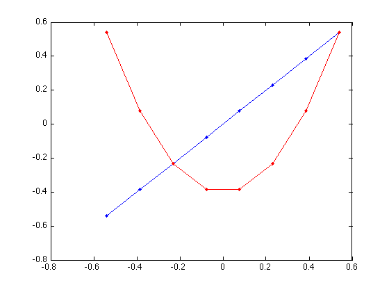
Linear trend analysis of boundary separation parameter a
Added by Nick 2010-10-20. All diffusion parameters come from the saturated model (aka MODEL_1). Revised by Alex 2010-20-22.
% We are only looking at the training portion (periods 1-8)
sbj=repmat((1:N_sbj)',1,N_periods_train) ;     % IV
period=repmat(1:N_periods_train,N_sbj,1) ;     % IV

% Run a standard ANOVA analsis on the first 8 periods
% We only want the first 8 points -- the training prior to the MAE and post-test
a27x8=B(1).a(:,1:N_periods_train) ;          % [N_sbj x N_periods], dependent var
[SS, df, MS, lbl] = anova(a27x8(:),[sbj(:) period(:)],'SP') ;

trend_a_ANOVA.labels = lbl' ;
trend_a_ANOVA.means = mean(a27x8) ;
trend_a_ANOVA.SS = SS' ;
trend_a_ANOVA.MS = MS' ;
trend_a_ANOVA.df = df' ;
trend_a_ANOVA.MS_err = MS(3) ;
trend_a_ANOVA.df_err = df(3) ;
trend_a_ANOVA.F_omnibus = MS(2)/MS(3) ;        % MS('P')/MS('SxP')
trend_a_ANOVA.p_omnibus = 1-fcdf(trend_a_ANOVA.F_omnibus,df(2),df(3)) ;

% Calculate effect size -- partial omega squared (KeppelWickens04, Sec.8.2)
% The partial omega squared estimates the *population* ratio
% sigma^2_effect / (sigma^2_effect + sigma^2_error)   (Eq.21.6),
% where sigma^2_error is the error variance for the particular effect.
F1 = max(0,trend_a_ANOVA.F_omnibus-1) ;  % Eq. 8.12 in KeppelWickens04
a1 = df(2)-1 ;
trend_a_ANOVA.omega2_omnibus = (a1*F1) / (a1*F1 + N_periods_train*N_sbj) ;

% Calculate the linear contrast
% Find psi-hat by summing over the products of each periods mean and its
% corresponding coefficient. The grand_mean.a is from the original 27 sbjs
%psi_hat = sum(lin_coef .* grand_means.a(1:N_periods_train)) ;
trend_a_ANOVA.linear_contrast_coefs = lin_coef ;
trend_a_ANOVA.psi_hat_linear = trend_a_ANOVA.means * lin_coef' ;

% Now we use equation 4.5 (pg 69) to complete the comparison
%SS_linear = (N_sbj*(psi_hat^2)) / sum((lin_coef.^2)) ;
trend_a_ANOVA.SS_linear = N_sbj * trend_a_ANOVA.psi_hat_linear^2 ;  % sum(coef.^2)==1

% Finally, we test for significance using the MS_error from the ANOVA
trend_a_ANOVA.F_linear = trend_a_ANOVA.SS_linear / trend_a_ANOVA.MS_err ;
trend_a_ANOVA.p_linear = 1-fcdf(trend_a_ANOVA.F_linear,1,trend_a_ANOVA.df_err) ;

% Calculate effect size -- partial omega squared (KeppelWickens04, Sec.8.2)
% For a contrast, the partial omega squared estimates the variability of
% the contrast relative to itself and the error rather than to all the
% variability in the study (p.165).  It is not affected by the size of any
% contrasts that are orthogonal to the contrast in question.
F1 = max(0,trend_a_ANOVA.F_linear-1) ;
trend_a_ANOVA.omega2_linear = F1 / (F1+2*N_sbj) ;  % Eq. 8.17 in KeppelWickens04


% We can evaluate the linear fit to see if it accounts for the variance seen
% See Eq. 4.16 in Keppel & Wickens (2004, p. 82)
trend_a_ANOVA.SS_failure_linear = trend_a_ANOVA.SS(2) - trend_a_ANOVA.SS_linear ;
trend_a_ANOVA.df_failure_linear = trend_a_ANOVA.df(2) - 1 ; % Linear trend has 1 df
trend_a_ANOVA.MS_failure_linear = trend_a_ANOVA.SS_failure_linear / trend_a_ANOVA.df_failure_linear ;
trend_a_ANOVA.F_failure_linear = trend_a_ANOVA.MS_failure_linear / trend_a_ANOVA.MS_err ;
trend_a_ANOVA.p_failure_linear = 1-fcdf(trend_a_ANOVA.F_failure_linear,...
                                        trend_a_ANOVA.df_failure_linear, trend_a_ANOVA.df_err)

% % Where F_{.05} =
% fprintf('F{.05} critical = %f, df=(%d,%d)\n', ...
%     finv(.95, trend_a_ANOVA.df_failure_linear, trend_a_ANOVA.df_err),...
%     trend_a_ANOVA.df_failure_linear, trend_a_ANOVA.df_err) ;
% % Where F_{.10} =
% fprintf('F{.10} critical = %f, df=(%d,%d)\n', ...
%     finv(.90, trend_a_ANOVA.df_failure_linear, trend_a_ANOVA.df_err),...
%     trend_a_ANOVA.df_failure_linear, trend_a_ANOVA.df_err) ;

% If F_failure_linear is not significant, then there is reason to doubt that
% a quadratic trend is necessary. However, one can check for this anyways (see below)

clear SS df MS lbl F1 a1
Partitioning the sum of squares...

 k Source         SumSq   eta2[%]     df        MeanSq
------------------------------------------------------
 1    S           0.113    49.91      26        0.0044
 2    P           0.007     3.04       7        0.0010
 3   SP           0.107    47.05     182        0.0006
 4  err           0.000     0.00       0        0.0000
 5 Totl           0.227   100.00     215        0.0011
------------------------------------------------------

trend_a_ANOVA =

                   labels: [4x5 char]
                    means: [0.1361 0.1415 0.1418 0.1316 0.1346 0.1292 0.1331 0.1238]
                       SS: [0.1133 0.0069 0.1068 1.7764e-15 0.2269]
                       MS: [0.0044 9.8560e-04 5.8656e-04 0 0.0011]
                       df: [26 7 182 0 215]
                   MS_err: 5.8656e-04
                   df_err: 182
                F_omnibus: 1.6803
                p_omnibus: 0.1163
           omega2_omnibus: 0.0185
    linear_contrast_coefs: [-0.5401 -0.3858 -0.2315 -0.0772 0.0772 0.2315 0.3858 0.5401]
           psi_hat_linear: -0.0126
                SS_linear: 0.0043
                 F_linear: 7.3228
                 p_linear: 0.0075
            omega2_linear: 0.1048
        SS_failure_linear: 0.0026
        df_failure_linear: 6
        MS_failure_linear: 4.3398e-04
         F_failure_linear: 0.7399
         p_failure_linear: 0.6182
Quadratic trend analysis of boundary separation parameter a
Added by Nick 2010-10-20. All diffusion parameters come from the saturated model (aka MODEL_1). Revised by Alex 2010-20-22.
% Calculate the quadratic contrast
% Find psi-hat by summing over the products of each periods mean and its
% corresponding coefficient
%psi_hat_quad = sum(quad_coef .* grand_means.a(1:N_periods_train)) ;
trend_a_ANOVA.quad_contrast_coefs = quad_coef ;
trend_a_ANOVA.psi_hat_quad = trend_a_ANOVA.means * quad_coef' ;

% Now we use equation 4.5 (pg 69) to complete the comparison
trend_a_ANOVA.SS_quad = N_sbj * trend_a_ANOVA.psi_hat_quad^2 ;  % sum(coef.^2)==1

% Finally, we test for significance using the MS_error from the ANOVA
trend_a_ANOVA.F_quad = trend_a_ANOVA.SS_quad / trend_a_ANOVA.MS_err ;
trend_a_ANOVA.p_quad = 1-fcdf(trend_a_ANOVA.F_quad,1,trend_a_ANOVA.df_err) ;

% Calculate partial omega squared for the quadratic contrast.  There must
% be a better way to do this. As it is now, the two effect sizes (linear +
% quadratic) can add up to more than 100%.
F1 = max(0,trend_a_ANOVA.F_quad-1) ;
trend_a_ANOVA.omega2_quad = F1 / (F1+2*N_sbj)   % Eq. 8.17 in KeppelWickens04
trend_a_ANOVA =

                   labels: [4x5 char]
                    means: [0.1361 0.1415 0.1418 0.1316 0.1346 0.1292 0.1331 0.1238]
                       SS: [0.1133 0.0069 0.1068 1.7764e-15 0.2269]
                       MS: [0.0044 9.8560e-04 5.8656e-04 0 0.0011]
                       df: [26 7 182 0 215]
                   MS_err: 5.8656e-04
                   df_err: 182
                F_omnibus: 1.6803
                p_omnibus: 0.1163
           omega2_omnibus: 0.0185
    linear_contrast_coefs: [-0.5401 -0.3858 -0.2315 -0.0772 0.0772 0.2315 0.3858 0.5401]
           psi_hat_linear: -0.0126
                SS_linear: 0.0043
                 F_linear: 7.3228
                 p_linear: 0.0075
            omega2_linear: 0.1048
        SS_failure_linear: 0.0026
        df_failure_linear: 6
        MS_failure_linear: 4.3398e-04
         F_failure_linear: 0.7399
         p_failure_linear: 0.6182
      quad_contrast_coefs: [0.5401 0.0772 -0.2315 -0.3858 -0.3858 -0.2315 0.0772 0.5401]
             psi_hat_quad: -0.0038
                  SS_quad: 3.9822e-04
                   F_quad: 0.6789
                   p_quad: 0.4110
              omega2_quad: 0
Linear (and quadratic) trend analysis of drift-stdev parameter eta
Added by Alex 2010-10-22. All diffusion parameters come from the saturated model (aka MODEL_1).
% % We are only looking at the training portion (periods 1-8)
% sbj=repmat((1:N_sbj)',1,N_periods_train) ;     % IV
% period=repmat(1:N_periods_train,N_sbj,1) ;     % IV

% Run a standard ANOVA analsis on the first 8 periods
% We only want the first 8 points -- the training prior to the MAE and post-test
eta27x8=B(1).eta(:,1:N_periods_train) ;  % [N_sbj x N_periods], dependent var
[SS, df, MS, lbl] = anova(eta27x8(:),[sbj(:) period(:)],'SP') ;

trend_eta_ANOVA.labels = lbl' ;
trend_eta_ANOVA.means = mean(eta27x8) ;
trend_eta_ANOVA.SS = SS' ;
trend_eta_ANOVA.MS = MS' ;
trend_eta_ANOVA.df = df' ;
trend_eta_ANOVA.MS_err = MS(3) ;
trend_eta_ANOVA.df_err = df(3) ;
trend_eta_ANOVA.F_omnibus = MS(2)/MS(3) ;        % MS('P')/MS('SxP')
trend_eta_ANOVA.p_omnibus = 1-fcdf(trend_eta_ANOVA.F_omnibus,df(2),df(3)) ;

% Calculate effect size -- partial omega squared (KeppelWickens04, Sec.8.2)
% The partial omega squared estimates the *population* ratio
% sigma^2_effect / (sigma^2_effect + sigma^2_error)   (Eq.21.6),
% where sigma^2_error is the error variance for the particular effect.
F1 = max(0,trend_eta_ANOVA.F_omnibus-1) ;  % Eq. 8.12 in KeppelWickens04
a1 = df(2)-1 ;
trend_eta_ANOVA.omega2_omnibus = (a1*F1) / (a1*F1 + N_periods_train*N_sbj) ;

% Calculate the linear contrast
% Find psi-hat by summing over the products of each periods mean and its
% corresponding coefficient. The grand_mean.a is from the original 27 sbjs
%psi_hat = sum(lin_coef .* grand_means.a(1:N_periods_train)) ;
trend_eta_ANOVA.linear_contrast_coefs = lin_coef ;
trend_eta_ANOVA.psi_hat_linear = trend_eta_ANOVA.means * lin_coef' ;

% Now we use equation 4.5 (pg 69) to complete the comparison
%SS_linear = (N_sbj*(psi_hat^2)) / sum((lin_coef.^2)) ;
trend_eta_ANOVA.SS_linear = N_sbj * trend_eta_ANOVA.psi_hat_linear^2 ;  % sum(coef.^2)==1

% Finally, we test for significance using the MS_error from the ANOVA
trend_eta_ANOVA.F_linear = trend_eta_ANOVA.SS_linear / trend_eta_ANOVA.MS_err ;
trend_eta_ANOVA.p_linear = 1-fcdf(trend_eta_ANOVA.F_linear,1,trend_eta_ANOVA.df_err) ;

% Calculate effect size -- partial omega squared (KeppelWickens04, Sec.8.2)
% For a contrast, the partial omega squared estimates the variability of
% the contrast relative to itself and the error rather than to all the
% variability in the study (p.165).  It is not affected by the size of any
% contrasts that are orthogonal to the contrast in question.
F1 = max(0,trend_eta_ANOVA.F_linear-1) ;
trend_eta_ANOVA.omega2_linear = F1 / (F1+2*N_sbj) ;  % Eq. 8.17 in KeppelWickens04


% We can evaluate the linear fit to see if it accounts for the variance seen
% See Eq. 4.16 in Keppel & Wickens (2004, p. 82)
trend_eta_ANOVA.SS_failure_linear = trend_eta_ANOVA.SS(2) - trend_eta_ANOVA.SS_linear ;
trend_eta_ANOVA.df_failure_linear = trend_eta_ANOVA.df(2) - 1 ; % Linear trend has 1 df
trend_eta_ANOVA.MS_failure_linear = trend_eta_ANOVA.SS_failure_linear / trend_eta_ANOVA.df_failure_linear ;
trend_eta_ANOVA.F_failure_linear = trend_eta_ANOVA.MS_failure_linear / trend_eta_ANOVA.MS_err ;
trend_eta_ANOVA.p_failure_linear = 1-fcdf(trend_eta_ANOVA.F_failure_linear,...
                                        trend_eta_ANOVA.df_failure_linear, trend_eta_ANOVA.df_err) ;

% Calculate the quadratic contrast
% Find psi-hat by summing over the products of each periods mean and its
% corresponding coefficient
%psi_hat_quad = sum(quad_coef .* grand_means.a(1:N_periods_train)) ;
trend_eta_ANOVA.quad_contrast_coefs = quad_coef ;
trend_eta_ANOVA.psi_hat_quad = trend_eta_ANOVA.means * quad_coef' ;

% Now we use equation 4.5 (pg 69) to complete the comparison
trend_eta_ANOVA.SS_quad = N_sbj * trend_eta_ANOVA.psi_hat_quad^2 ;  % sum(coef.^2)==1

% Finally, we test for significance using the MS_error from the ANOVA
trend_eta_ANOVA.F_quad = trend_eta_ANOVA.SS_quad / trend_eta_ANOVA.MS_err ;
trend_eta_ANOVA.p_quad = 1-fcdf(trend_eta_ANOVA.F_quad,1,trend_eta_ANOVA.df_err) ;

% Calculate partial omega squared for the quadratic contrast.  There must
% be a better way to do this. As it is now, the two effect sizes (linear +
% quadratic) can add up to more than 100%.
F1 = max(0,trend_eta_ANOVA.F_quad-1) ;
trend_eta_ANOVA.omega2_quad = F1 / (F1+2*N_sbj)   % Eq. 8.17 in KeppelWickens04

clear SS df MS lbl F1 a1
Partitioning the sum of squares...

 k Source         SumSq   eta2[%]     df        MeanSq
------------------------------------------------------
 1    S           0.423    21.76      26        0.0163
 2    P           0.109     5.59       7        0.0155
 3   SP           1.411    72.65     182        0.0078
 4  err          -0.000    -0.00       0        0.0000
 5 Totl           1.942   100.00     215        0.0090
------------------------------------------------------

trend_eta_ANOVA =

                   labels: [4x5 char]
                    means: [0.1974 0.2446 0.2556 0.2412 0.2765 0.2433 0.2500 0.2707]
                       SS: [0.4226 0.1086 1.4108 -7.1054e-15 1.9420]
                       MS: [0.0163 0.0155 0.0078 0 0.0090]
                       df: [26 7 182 0 215]
                   MS_err: 0.0078
                   df_err: 182
                F_omnibus: 2.0015
                p_omnibus: 0.0572
           omega2_omnibus: 0.0271
    linear_contrast_coefs: [-0.5401 -0.3858 -0.2315 -0.0772 0.0772 0.2315 0.3858 0.5401]
           psi_hat_linear: 0.0415
                SS_linear: 0.0465
                 F_linear: 6.0054
                 p_linear: 0.0152
            omega2_linear: 0.0848
        SS_failure_linear: 0.0621
        df_failure_linear: 6
        MS_failure_linear: 0.0103
         F_failure_linear: 1.3342
         p_failure_linear: 0.2441
      quad_contrast_coefs: [0.5401 0.0772 -0.2315 -0.3858 -0.3858 -0.2315 0.0772 0.5401]
             psi_hat_quad: -0.0242
                  SS_quad: 0.0158
                   F_quad: 2.0380
                   p_quad: 0.1551
              omega2_quad: 0.0189
Linear (and quadratic) trend analysis of starting-point range parameter sz
Added by Alex 2010-10-22. All diffusion parameters come from the saturated model (aka MODEL_1).
% % We are only looking at the training portion (periods 1-8)
% sbj=repmat((1:N_sbj)',1,N_periods_train) ;     % IV
% period=repmat(1:N_periods_train,N_sbj,1) ;     % IV

% Run a standard ANOVA analsis on the first 8 periods
% We only want the first 8 points -- the training prior to the MAE and post-test
sz27x8=B(1).sz(:,1:N_periods_train) ;  % [N_sbj x N_periods], dependent var
[SS, df, MS, lbl] = anova(sz27x8(:),[sbj(:) period(:)],'SP') ;

trend_sz_ANOVA.labels = lbl' ;
trend_sz_ANOVA.means = mean(sz27x8) ;
trend_sz_ANOVA.SS = SS' ;
trend_sz_ANOVA.MS = MS' ;
trend_sz_ANOVA.df = df' ;
trend_sz_ANOVA.MS_err = MS(3) ;
trend_sz_ANOVA.df_err = df(3) ;
trend_sz_ANOVA.F_omnibus = MS(2)/MS(3) ;        % MS('P')/MS('SxP')
trend_sz_ANOVA.p_omnibus = 1-fcdf(trend_sz_ANOVA.F_omnibus,df(2),df(3)) ;

% Calculate effect size -- partial omega squared (KeppelWickens04, Sec.8.2)
% The partial omega squared estimates the *population* ratio
% sigma^2_effect / (sigma^2_effect + sigma^2_error)   (Eq.21.6),
% where sigma^2_error is the error variance for the particular effect.
F1 = max(0,trend_sz_ANOVA.F_omnibus-1) ;  % Eq. 8.12 in KeppelWickens04
a1 = df(2)-1 ;
trend_sz_ANOVA.omega2_omnibus = (a1*F1) / (a1*F1 + N_periods_train*N_sbj) ;

% Calculate the linear contrast
% Find psi-hat by summing over the products of each periods mean and its
% corresponding coefficient. The grand_mean.a is from the original 27 sbjs
%psi_hat = sum(lin_coef .* grand_means.a(1:N_periods_train)) ;
trend_sz_ANOVA.linear_contrast_coefs = lin_coef ;
trend_sz_ANOVA.psi_hat_linear = trend_sz_ANOVA.means * lin_coef' ;

% Now we use equation 4.5 (pg 69) to complete the comparison
%SS_linear = (N_sbj*(psi_hat^2)) / sum((lin_coef.^2)) ;
trend_sz_ANOVA.SS_linear = N_sbj * trend_sz_ANOVA.psi_hat_linear^2 ;  % sum(coef.^2)==1

% Finally, we test for significance using the MS_error from the ANOVA
trend_sz_ANOVA.F_linear = trend_sz_ANOVA.SS_linear / trend_sz_ANOVA.MS_err ;
trend_sz_ANOVA.p_linear = 1-fcdf(trend_sz_ANOVA.F_linear,1,trend_sz_ANOVA.df_err) ;

% Calculate effect size -- partial omega squared (KeppelWickens04, Sec.8.2)
% For a contrast, the partial omega squared estimates the variability of
% the contrast relative to itself and the error rather than to all the
% variability in the study (p.165).  It is not affected by the size of any
% contrasts that are orthogonal to the contrast in question.
F1 = max(0,trend_sz_ANOVA.F_linear-1) ;
trend_sz_ANOVA.omega2_linear = F1 / (F1+2*N_sbj) ;  % Eq. 8.17 in KeppelWickens04


% We can evaluate the linear fit to see if it accounts for the variance seen
% See Eq. 4.16 in Keppel & Wickens (2004, p. 82)
trend_sz_ANOVA.SS_failure_linear = trend_sz_ANOVA.SS(2) - trend_sz_ANOVA.SS_linear ;
trend_sz_ANOVA.df_failure_linear = trend_sz_ANOVA.df(2) - 1 ; % Linear trend has 1 df
trend_sz_ANOVA.MS_failure_linear = trend_sz_ANOVA.SS_failure_linear / trend_sz_ANOVA.df_failure_linear ;
trend_sz_ANOVA.F_failure_linear = trend_sz_ANOVA.MS_failure_linear / trend_sz_ANOVA.MS_err ;
trend_sz_ANOVA.p_failure_linear = 1-fcdf(trend_sz_ANOVA.F_failure_linear,...
                                        trend_sz_ANOVA.df_failure_linear, trend_sz_ANOVA.df_err) ;

% Calculate the quadratic contrast
% Find psi-hat by summing over the products of each periods mean and its
% corresponding coefficient
%psi_hat_quad = sum(quad_coef .* grand_means.a(1:N_periods_train)) ;
trend_sz_ANOVA.quad_contrast_coefs = quad_coef ;
trend_sz_ANOVA.psi_hat_quad = trend_sz_ANOVA.means * quad_coef' ;

% Now we use equation 4.5 (pg 69) to complete the comparison
trend_sz_ANOVA.SS_quad = N_sbj * trend_sz_ANOVA.psi_hat_quad^2 ;  % sum(coef.^2)==1

% Finally, we test for significance using the MS_error from the ANOVA
trend_sz_ANOVA.F_quad = trend_sz_ANOVA.SS_quad / trend_sz_ANOVA.MS_err ;
trend_sz_ANOVA.p_quad = 1-fcdf(trend_sz_ANOVA.F_quad,1,trend_sz_ANOVA.df_err) ;

% Calculate partial omega squared for the quadratic contrast.  There must
% be a better way to do this. As it is now, the two effect sizes (linear +
% quadratic) can add up to more than 100%.
F1 = max(0,trend_sz_ANOVA.F_quad-1) ;
trend_sz_ANOVA.omega2_quad = F1 / (F1+2*N_sbj)   % Eq. 8.17 in KeppelWickens04

clear SS df MS lbl F1 a1
Partitioning the sum of squares...

 k Source         SumSq   eta2[%]     df        MeanSq
------------------------------------------------------
 1    S           0.071    27.26      26        0.0027
 2    P           0.008     3.21       7        0.0012
 3   SP           0.180    69.53     182        0.0010
 4  err           0.000     0.00       0        0.0000
 5 Totl           0.259   100.00     215        0.0012
------------------------------------------------------

trend_sz_ANOVA =

                   labels: [4x5 char]
                    means: [0.0454 0.0458 0.0353 0.0407 0.0570 0.0521 0.0440 0.0440]
                       SS: [0.0705 0.0083 0.1799 4.4409e-16 0.2587]
                       MS: [0.0027 0.0012 9.8836e-04 0 0.0012]
                       df: [26 7 182 0 215]
                   MS_err: 9.8836e-04
                   df_err: 182
                F_omnibus: 1.2007
                p_omnibus: 0.3045
           omega2_omnibus: 0.0055
    linear_contrast_coefs: [-0.5401 -0.3858 -0.2315 -0.0772 0.0772 0.2315 0.3858 0.5401]
           psi_hat_linear: 0.0037
                SS_linear: 3.6176e-04
                 F_linear: 0.3660
                 p_linear: 0.5459
            omega2_linear: 0
        SS_failure_linear: 0.0079
        df_failure_linear: 6
        MS_failure_linear: 0.0013
         F_failure_linear: 1.3398
         p_failure_linear: 0.2416
      quad_contrast_coefs: [0.5401 0.0772 -0.2315 -0.3858 -0.3858 -0.2315 0.0772 0.5401]
             psi_hat_quad: -0.0027
                  SS_quad: 1.9771e-04
                   F_quad: 0.2000
                   p_quad: 0.6552
              omega2_quad: 0
Linear (and quadratic) trend analysis of easy drift rate v1
Added by Alex 2010-10-22. All diffusion parameters come from the saturated model (aka MODEL_1).
% % We are only looking at the training portion (periods 1-8)
% sbj=repmat((1:N_sbj)',1,N_periods_train) ;     % IV
% period=repmat(1:N_periods_train,N_sbj,1) ;     % IV

% Run a standard ANOVA analsis on the first 8 periods
% We only want the first 8 points -- the training prior to the MAE and post-test
v1_27x8=B(1).v1(:,1:N_periods_train) ;  % [N_sbj x N_periods], dependent var
[SS, df, MS, lbl] = anova(v1_27x8(:),[sbj(:) period(:)],'SP') ;

trend_v1_ANOVA.labels = lbl' ;
trend_v1_ANOVA.means = mean(v1_27x8) ;
trend_v1_ANOVA.SS = SS' ;
trend_v1_ANOVA.MS = MS' ;
trend_v1_ANOVA.df = df' ;
trend_v1_ANOVA.MS_err = MS(3) ;
trend_v1_ANOVA.df_err = df(3) ;
trend_v1_ANOVA.F_omnibus = MS(2)/MS(3) ;        % MS('P')/MS('SxP')
trend_v1_ANOVA.p_omnibus = 1-fcdf(trend_v1_ANOVA.F_omnibus,df(2),df(3)) ;

% Calculate effect size -- partial omega squared (KeppelWickens04, Sec.8.2)
% The partial omega squared estimates the *population* ratio
% sigma^2_effect / (sigma^2_effect + sigma^2_error)   (Eq.21.6),
% where sigma^2_error is the error variance for the particular effect.
F1 = max(0,trend_v1_ANOVA.F_omnibus-1) ;  % Eq. 8.12 in KeppelWickens04
a1 = df(2)-1 ;
trend_v1_ANOVA.omega2_omnibus = (a1*F1) / (a1*F1 + N_periods_train*N_sbj) ;

% Calculate the linear contrast
% Find psi-hat by summing over the products of each periods mean and its
% corresponding coefficient. The grand_mean.a is from the original 27 sbjs
%psi_hat = sum(lin_coef .* grand_means.a(1:N_periods_train)) ;
trend_v1_ANOVA.linear_contrast_coefs = lin_coef ;
trend_v1_ANOVA.psi_hat_linear = trend_v1_ANOVA.means * lin_coef' ;

% Now we use equation 4.5 (pg 69) to complete the comparison
%SS_linear = (N_sbj*(psi_hat^2)) / sum((lin_coef.^2)) ;
trend_v1_ANOVA.SS_linear = N_sbj * trend_v1_ANOVA.psi_hat_linear^2 ;  % sum(coef.^2)==1

% Finally, we test for significance using the MS_error from the ANOVA
trend_v1_ANOVA.F_linear = trend_v1_ANOVA.SS_linear / trend_v1_ANOVA.MS_err ;
trend_v1_ANOVA.p_linear = 1-fcdf(trend_v1_ANOVA.F_linear,1,trend_v1_ANOVA.df_err) ;

% Calculate effect size -- partial omega squared (KeppelWickens04, Sec.8.2)
% For a contrast, the partial omega squared estimates the variability of
% the contrast relative to itself and the error rather than to all the
% variability in the study (p.165).  It is not affected by the size of any
% contrasts that are orthogonal to the contrast in question.
F1 = max(0,trend_v1_ANOVA.F_linear-1) ;
trend_v1_ANOVA.omega2_linear = F1 / (F1+2*N_sbj) ;  % Eq. 8.17 in KeppelWickens04


% We can evaluate the linear fit to see if it accounts for the variance seen
% See Eq. 4.16 in Keppel & Wickens (2004, p. 82)
trend_v1_ANOVA.SS_failure_linear = trend_v1_ANOVA.SS(2) - trend_v1_ANOVA.SS_linear ;
trend_v1_ANOVA.df_failure_linear = trend_v1_ANOVA.df(2) - 1 ; % Linear trend has 1 df
trend_v1_ANOVA.MS_failure_linear = trend_v1_ANOVA.SS_failure_linear / trend_v1_ANOVA.df_failure_linear ;
trend_v1_ANOVA.F_failure_linear = trend_v1_ANOVA.MS_failure_linear / trend_v1_ANOVA.MS_err ;
trend_v1_ANOVA.p_failure_linear = 1-fcdf(trend_v1_ANOVA.F_failure_linear,...
                                        trend_v1_ANOVA.df_failure_linear, trend_v1_ANOVA.df_err) ;

% Calculate the quadratic contrast
% Find psi-hat by summing over the products of each periods mean and its
% corresponding coefficient
%psi_hat_quad = sum(quad_coef .* grand_means.a(1:N_periods_train)) ;
trend_v1_ANOVA.quad_contrast_coefs = quad_coef ;
trend_v1_ANOVA.psi_hat_quad = trend_v1_ANOVA.means * quad_coef' ;

% Now we use equation 4.5 (pg 69) to complete the comparison
trend_v1_ANOVA.SS_quad = N_sbj * trend_v1_ANOVA.psi_hat_quad^2 ;  % sum(coef.^2)==1

% Finally, we test for significance using the MS_error from the ANOVA
trend_v1_ANOVA.F_quad = trend_v1_ANOVA.SS_quad / trend_v1_ANOVA.MS_err ;
trend_v1_ANOVA.p_quad = 1-fcdf(trend_v1_ANOVA.F_quad,1,trend_v1_ANOVA.df_err) ;

% Calculate partial omega squared for the quadratic contrast.  There must
% be a better way to do this. As it is now, the two effect sizes (linear +
% quadratic) can add up to more than 100%.
F1 = max(0,trend_v1_ANOVA.F_quad-1) ;
trend_v1_ANOVA.omega2_quad = F1 / (F1+2*N_sbj)   % Eq. 8.17 in KeppelWickens04


clear SS df MS lbl F1 a1
Partitioning the sum of squares...

 k Source         SumSq   eta2[%]     df        MeanSq
------------------------------------------------------
 1    S           2.222    42.49      26        0.0855
 2    P           1.114    21.31       7        0.1592
 3   SP           1.894    36.21     182        0.0104
 4  err          -0.000    -0.00       0        0.0000
 5 Totl           5.230   100.00     215        0.0243
------------------------------------------------------

trend_v1_ANOVA =

                   labels: [4x5 char]
                    means: [0.2541 0.3517 0.3980 0.4133 0.4546 0.4477 0.4588 0.4973]
                       SS: [2.2219 1.1144 1.8935 -1.4211e-14 5.2298]
                       MS: [0.0855 0.1592 0.0104 0 0.0243]
                       df: [26 7 182 0 215]
                   MS_err: 0.0104
                   df_err: 182
                F_omnibus: 15.3016
                p_omnibus: 1.1102e-15
           omega2_omnibus: 0.2843
    linear_contrast_coefs: [-0.5401 -0.3858 -0.2315 -0.0772 0.0772 0.2315 0.3858 0.5401]
           psi_hat_linear: 0.1873
                SS_linear: 0.9477
                 F_linear: 91.0905
                 p_linear: 0
            omega2_linear: 0.6252
        SS_failure_linear: 0.1667
        df_failure_linear: 6
        MS_failure_linear: 0.0278
         F_failure_linear: 2.6701
         p_failure_linear: 0.0166
      quad_contrast_coefs: [0.5401 0.0772 -0.2315 -0.3858 -0.3858 -0.2315 0.0772 0.5401]
             psi_hat_quad: -0.0622
                  SS_quad: 0.1046
                   F_quad: 10.0509
                   p_quad: 0.0018
              omega2_quad: 0.1435
Linear (and quadratic) trend analysis of difficult drift rate v2
Added by Alex 2010-10-22. All diffusion parameters come from the saturated model (aka MODEL_1).
% % We are only looking at the training portion (periods 1-8)
% sbj=repmat((1:N_sbj)',1,N_periods_train) ;     % IV
% period=repmat(1:N_periods_train,N_sbj,1) ;     % IV

% Run a standard ANOVA analsis on the first 8 periods
% We only want the first 8 points -- the training prior to the MAE and post-test
v2_27x8=B(1).v2(:,1:N_periods_train) ;  % [N_sbj x N_periods], dependent var
[SS, df, MS, lbl] = anova(v2_27x8(:),[sbj(:) period(:)],'SP') ;

trend_v2_ANOVA.labels = lbl' ;
trend_v2_ANOVA.means = mean(v2_27x8) ;
trend_v2_ANOVA.SS = SS' ;
trend_v2_ANOVA.MS = MS' ;
trend_v2_ANOVA.df = df' ;
trend_v2_ANOVA.MS_err = MS(3) ;
trend_v2_ANOVA.df_err = df(3) ;
trend_v2_ANOVA.F_omnibus = MS(2)/MS(3) ;        % MS('P')/MS('SxP')
trend_v2_ANOVA.p_omnibus = 1-fcdf(trend_v2_ANOVA.F_omnibus,df(2),df(3)) ;

% Calculate effect size -- partial omega squared (KeppelWickens04, Sec.8.2)
% The partial omega squared estimates the *population* ratio
% sigma^2_effect / (sigma^2_effect + sigma^2_error)   (Eq.21.6),
% where sigma^2_error is the error variance for the particular effect.
F1 = max(0,trend_v2_ANOVA.F_omnibus-1) ;  % Eq. 8.12 in KeppelWickens04
a1 = df(2)-1 ;
trend_v2_ANOVA.omega2_omnibus = (a1*F1) / (a1*F1 + N_periods_train*N_sbj) ;

% Calculate the linear contrast
% Find psi-hat by summing over the products of each periods mean and its
% corresponding coefficient. The grand_mean.a is from the original 27 sbjs
%psi_hat = sum(lin_coef .* grand_means.a(1:N_periods_train)) ;
trend_v2_ANOVA.linear_contrast_coefs = lin_coef ;
trend_v2_ANOVA.psi_hat_linear = trend_v2_ANOVA.means * lin_coef' ;

% Now we use equation 4.5 (pg 69) to complete the comparison
%SS_linear = (N_sbj*(psi_hat^2)) / sum((lin_coef.^2)) ;
trend_v2_ANOVA.SS_linear = N_sbj * trend_v2_ANOVA.psi_hat_linear^2 ;  % sum(coef.^2)==1

% Finally, we test for significance using the MS_error from the ANOVA
trend_v2_ANOVA.F_linear = trend_v2_ANOVA.SS_linear / trend_v2_ANOVA.MS_err ;
trend_v2_ANOVA.p_linear = 1-fcdf(trend_v2_ANOVA.F_linear,1,trend_v2_ANOVA.df_err) ;

% Calculate effect size -- partial omega squared (KeppelWickens04, Sec.8.2)
% For a contrast, the partial omega squared estimates the variability of
% the contrast relative to itself and the error rather than to all the
% variability in the study (p.165).  It is not affected by the size of any
% contrasts that are orthogonal to the contrast in question.
F1 = max(0,trend_v2_ANOVA.F_linear-1) ;
trend_v2_ANOVA.omega2_linear = F1 / (F1+2*N_sbj) ;  % Eq. 8.17 in KeppelWickens04


% We can evaluate the linear fit to see if it accounts for the variance seen
% See Eq. 4.16 in Keppel & Wickens (2004, p. 82)
trend_v2_ANOVA.SS_failure_linear = trend_v2_ANOVA.SS(2) - trend_v2_ANOVA.SS_linear ;
trend_v2_ANOVA.df_failure_linear = trend_v2_ANOVA.df(2) - 1 ; % Linear trend has 1 df
trend_v2_ANOVA.MS_failure_linear = trend_v2_ANOVA.SS_failure_linear / trend_v2_ANOVA.df_failure_linear ;
trend_v2_ANOVA.F_failure_linear = trend_v2_ANOVA.MS_failure_linear / trend_v2_ANOVA.MS_err ;
trend_v2_ANOVA.p_failure_linear = 1-fcdf(trend_v2_ANOVA.F_failure_linear,...
                                        trend_v2_ANOVA.df_failure_linear, trend_v2_ANOVA.df_err) ;

% Calculate the quadratic contrast
% Find psi-hat by summing over the products of each periods mean and its
% corresponding coefficient
%psi_hat_quad = sum(quad_coef .* grand_means.a(1:N_periods_train)) ;
trend_v2_ANOVA.quad_contrast_coefs = quad_coef ;
trend_v2_ANOVA.psi_hat_quad = trend_v2_ANOVA.means * quad_coef' ;

% Now we use equation 4.5 (pg 69) to complete the comparison
trend_v2_ANOVA.SS_quad = N_sbj * trend_v2_ANOVA.psi_hat_quad^2 ;  % sum(coef.^2)==1

% Finally, we test for significance using the MS_error from the ANOVA
trend_v2_ANOVA.F_quad = trend_v2_ANOVA.SS_quad / trend_v2_ANOVA.MS_err ;
trend_v2_ANOVA.p_quad = 1-fcdf(trend_v2_ANOVA.F_quad,1,trend_v2_ANOVA.df_err) ;

% Calculate partial omega squared for the quadratic contrast.  There must
% be a better way to do this. As it is now, the two effect sizes (linear +
% quadratic) can add up to more than 100%.
F1 = max(0,trend_v2_ANOVA.F_quad-1) ;
trend_v2_ANOVA.omega2_quad = F1 / (F1+2*N_sbj)   % Eq. 8.17 in KeppelWickens04

clear SS df MS lbl F1 a1
Partitioning the sum of squares...

 k Source         SumSq   eta2[%]     df        MeanSq
------------------------------------------------------
 1    S           1.022    45.18      26        0.0393
 2    P           0.468    20.68       7        0.0668
 3   SP           0.773    34.14     182        0.0042
 4  err          -0.000    -0.00       0        0.0000
 5 Totl           2.262   100.00     215        0.0105
------------------------------------------------------

trend_v2_ANOVA =

                   labels: [4x5 char]
                    means: [0.1477 0.2118 0.2311 0.2497 0.2776 0.2769 0.2798 0.3023]
                       SS: [1.0221 0.4679 0.7725 -7.1054e-15 2.2625]
                       MS: [0.0393 0.0668 0.0042 0 0.0105]
                       df: [26 7 182 0 215]
                   MS_err: 0.0042
                   df_err: 182
                F_omnibus: 15.7463
                p_omnibus: 4.4409e-16
           omega2_omnibus: 0.2906
    linear_contrast_coefs: [-0.5401 -0.3858 -0.2315 -0.0772 0.0772 0.2315 0.3858 0.5401]
           psi_hat_linear: 0.1225
                SS_linear: 0.4052
                 F_linear: 95.4601
                 p_linear: 0
            omega2_linear: 0.6363
        SS_failure_linear: 0.0627
        df_failure_linear: 6
        MS_failure_linear: 0.0104
         F_failure_linear: 2.4607
         p_failure_linear: 0.0260
      quad_contrast_coefs: [0.5401 0.0772 -0.2315 -0.3858 -0.3858 -0.2315 0.0772 0.5401]
             psi_hat_quad: -0.0400
                  SS_quad: 0.0432
                   F_quad: 10.1844
                   p_quad: 0.0017
              omega2_quad: 0.1454
Linear (and quadratic) trend analysis of the average drift rate v_avg
Added by Alex 2010-10-22. All diffusion parameters come from the saturated model (aka MODEL_1).
% % We are only looking at the training portion (periods 1-8)
% sbj=repmat((1:N_sbj)',1,N_periods_train) ;     % IV
% period=repmat(1:N_periods_train,N_sbj,1) ;     % IV

% Run a standard ANOVA analsis on the first 8 periods
% We only want the first 8 points -- the training prior to the MAE and post-test
v_avg_27x8=B(1).v_avg(:,1:N_periods_train) ;  % [N_sbj x N_periods], dependent var
[SS, df, MS, lbl] = anova(v_avg_27x8(:),[sbj(:) period(:)],'SP') ;

trend_v_avg_ANOVA.labels = lbl' ;
trend_v_avg_ANOVA.means = mean(v_avg_27x8) ;
trend_v_avg_ANOVA.SS = SS' ;
trend_v_avg_ANOVA.MS = MS' ;
trend_v_avg_ANOVA.df = df' ;
trend_v_avg_ANOVA.MS_err = MS(3) ;
trend_v_avg_ANOVA.df_err = df(3) ;
trend_v_avg_ANOVA.F_omnibus = MS(2)/MS(3) ;        % MS('P')/MS('SxP')
trend_v_avg_ANOVA.p_omnibus = 1-fcdf(trend_v_avg_ANOVA.F_omnibus,df(2),df(3)) ;

% Calculate effect size -- partial omega squared (KeppelWickens04, Sec.8.2)
% The partial omega squared estimates the *population* ratio
% sigma^2_effect / (sigma^2_effect + sigma^2_error)   (Eq.21.6),
% where sigma^2_error is the error variance for the particular effect.
F1 = max(0,trend_v_avg_ANOVA.F_omnibus-1) ;  % Eq. 8.12 in KeppelWickens04
a1 = df(2)-1 ;
trend_v_avg_ANOVA.omega2_omnibus = (a1*F1) / (a1*F1 + N_periods_train*N_sbj) ;

% Calculate the linear contrast
% Find psi-hat by summing over the products of each periods mean and its
% corresponding coefficient. The grand_mean.a is from the original 27 sbjs
%psi_hat = sum(lin_coef .* grand_means.a(1:N_periods_train)) ;
trend_v_avg_ANOVA.linear_contrast_coefs = lin_coef ;
trend_v_avg_ANOVA.psi_hat_linear = trend_v_avg_ANOVA.means * lin_coef' ;

% Now we use equation 4.5 (pg 69) to complete the comparison
%SS_linear = (N_sbj*(psi_hat^2)) / sum((lin_coef.^2)) ;
trend_v_avg_ANOVA.SS_linear = N_sbj * trend_v_avg_ANOVA.psi_hat_linear^2 ;  % sum(coef.^2)==1

% Finally, we test for significance using the MS_error from the ANOVA
trend_v_avg_ANOVA.F_linear = trend_v_avg_ANOVA.SS_linear / trend_v_avg_ANOVA.MS_err ;
trend_v_avg_ANOVA.p_linear = 1-fcdf(trend_v_avg_ANOVA.F_linear,1,trend_v_avg_ANOVA.df_err) ;

% Calculate effect size -- partial omega squared (KeppelWickens04, Sec.8.2)
% For a contrast, the partial omega squared estimates the variability of
% the contrast relative to itself and the error rather than to all the
% variability in the study (p.165).  It is not affected by the size of any
% contrasts that are orthogonal to the contrast in question.
F1 = max(0,trend_v_avg_ANOVA.F_linear-1) ;
trend_v_avg_ANOVA.omega2_linear = F1 / (F1+2*N_sbj) ;  % Eq. 8.17 in KeppelWickens04


% We can evaluate the linear fit to see if it accounts for the variance seen
% See Eq. 4.16 in Keppel & Wickens (2004, p. 82)
trend_v_avg_ANOVA.SS_failure_linear = trend_v_avg_ANOVA.SS(2) - trend_v_avg_ANOVA.SS_linear ;
trend_v_avg_ANOVA.df_failure_linear = trend_v_avg_ANOVA.df(2) - 1 ; % Linear trend has 1 df
trend_v_avg_ANOVA.MS_failure_linear = trend_v_avg_ANOVA.SS_failure_linear / trend_v_avg_ANOVA.df_failure_linear ;
trend_v_avg_ANOVA.F_failure_linear = trend_v_avg_ANOVA.MS_failure_linear / trend_v_avg_ANOVA.MS_err ;
trend_v_avg_ANOVA.p_failure_linear = 1-fcdf(trend_v_avg_ANOVA.F_failure_linear,...
                                        trend_v_avg_ANOVA.df_failure_linear, trend_v_avg_ANOVA.df_err) ;

% Calculate the quadratic contrast
% Find psi-hat by summing over the products of each periods mean and its
% corresponding coefficient
%psi_hat_quad = sum(quad_coef .* grand_means.a(1:N_periods_train)) ;
trend_v_avg_ANOVA.quad_contrast_coefs = quad_coef ;
trend_v_avg_ANOVA.psi_hat_quad = trend_v_avg_ANOVA.means * quad_coef' ;

% Now we use equation 4.5 (pg 69) to complete the comparison
trend_v_avg_ANOVA.SS_quad = N_sbj * trend_v_avg_ANOVA.psi_hat_quad^2 ;  % sum(coef.^2)==1

% Finally, we test for significance using the MS_error from the ANOVA
trend_v_avg_ANOVA.F_quad = trend_v_avg_ANOVA.SS_quad / trend_v_avg_ANOVA.MS_err ;
trend_v_avg_ANOVA.p_quad = 1-fcdf(trend_v_avg_ANOVA.F_quad,1,trend_v_avg_ANOVA.df_err) ;

% Calculate partial omega squared for the quadratic contrast.  There must
% be a better way to do this. As it is now, the two effect sizes (linear +
% quadratic) can add up to more than 100%.
F1 = max(0,trend_v_avg_ANOVA.F_quad-1) ;
trend_v_avg_ANOVA.omega2_quad = F1 / (F1+2*N_sbj)   % Eq. 8.17 in KeppelWickens04

clear SS df MS lbl F1 a1
Partitioning the sum of squares...

 k Source         SumSq   eta2[%]     df        MeanSq
------------------------------------------------------
 1    S           1.554    44.27      26        0.0598
 2    P           0.755    21.52       7        0.1079
 3   SP           1.201    34.21     182        0.0066
 4  err          -0.000    -0.00       0        0.0000
 5 Totl           3.510   100.00     215        0.0163
------------------------------------------------------

trend_v_avg_ANOVA =

                   labels: [4x5 char]
                    means: [0.2009 0.2818 0.3145 0.3315 0.3661 0.3623 0.3693 0.3998]
                       SS: [1.5540 0.7555 1.2009 -3.5527e-15 3.5104]
                       MS: [0.0598 0.1079 0.0066 0 0.0163]
                       df: [26 7 182 0 215]
                   MS_err: 0.0066
                   df_err: 182
                F_omnibus: 16.3552
                p_omnibus: 1.1102e-16
           omega2_omnibus: 0.2990
    linear_contrast_coefs: [-0.5401 -0.3858 -0.2315 -0.0772 0.0772 0.2315 0.3858 0.5401]
           psi_hat_linear: 0.1549
                SS_linear: 0.6481
                 F_linear: 98.2111
                 p_linear: 0
            omega2_linear: 0.6429
        SS_failure_linear: 0.1074
        df_failure_linear: 6
        MS_failure_linear: 0.0179
         F_failure_linear: 2.7126
         p_failure_linear: 0.0151
      quad_contrast_coefs: [0.5401 0.0772 -0.2315 -0.3858 -0.3858 -0.2315 0.0772 0.5401]
             psi_hat_quad: -0.0511
                  SS_quad: 0.0706
                   F_quad: 10.6941
                   p_quad: 0.0013
              omega2_quad: 0.1522
Linear (and quadratic) trend analysis of the average dprime
Added by Alex 2010-11-10.
% % We are only looking at the training portion (periods 1-8)
% sbj=repmat((1:N_sbj)',1,N_periods_train) ;     % IV
% period=repmat(1:N_periods_train,N_sbj,1) ;     % IV

% Run a standard ANOVA analsis on the first 8 periods
% We only want the first 8 points -- the training prior to the MAE and post-test
dpr_avg_27x8 = dp11(1:N_periods_train,:)' ;  % [N_sbj x N_periods], dependent var
[SS, df, MS, lbl] = anova(dpr_avg_27x8(:),[sbj(:) period(:)],'SP') ;

trend_dpr_avg_ANOVA.labels = lbl' ;
trend_dpr_avg_ANOVA.means = mean(dpr_avg_27x8) ;
trend_dpr_avg_ANOVA.SS = SS' ;
trend_dpr_avg_ANOVA.MS = MS' ;
trend_dpr_avg_ANOVA.df = df' ;
trend_dpr_avg_ANOVA.MS_err = MS(3) ;
trend_dpr_avg_ANOVA.df_err = df(3) ;
trend_dpr_avg_ANOVA.F_omnibus = MS(2)/MS(3) ;        % MS('P')/MS('SxP')
trend_dpr_avg_ANOVA.p_omnibus = 1-fcdf(trend_dpr_avg_ANOVA.F_omnibus,df(2),df(3)) ;

% Calculate effect size -- partial omega squared (KeppelWickens04, Sec.8.2)
% The partial omega squared estimates the *population* ratio
% sigma^2_effect / (sigma^2_effect + sigma^2_error)   (Eq.21.6),
% where sigma^2_error is the error variance for the particular effect.
F1 = max(0,trend_dpr_avg_ANOVA.F_omnibus-1) ;  % Eq. 8.12 in KeppelWickens04
a1 = df(2)-1 ;
trend_dpr_avg_ANOVA.omega2_omnibus = (a1*F1) / (a1*F1 + N_periods_train*N_sbj) ;

% Calculate the linear contrast
% Find psi-hat by summing over the products of each periods mean and its
% corresponding coefficient. The grand_mean.a is from the original 27 sbjs
%psi_hat = sum(lin_coef .* grand_means.a(1:N_periods_train)) ;
trend_dpr_avg_ANOVA.linear_contrast_coefs = lin_coef ;
trend_dpr_avg_ANOVA.psi_hat_linear = trend_dpr_avg_ANOVA.means * lin_coef' ;

% Now we use equation 4.5 (pg 69) to complete the comparison
%SS_linear = (N_sbj*(psi_hat^2)) / sum((lin_coef.^2)) ;
trend_dpr_avg_ANOVA.SS_linear = N_sbj * trend_dpr_avg_ANOVA.psi_hat_linear^2 ;  % sum(coef.^2)==1

% Finally, we test for significance using the MS_error from the ANOVA
trend_dpr_avg_ANOVA.F_linear = trend_dpr_avg_ANOVA.SS_linear / trend_dpr_avg_ANOVA.MS_err ;
trend_dpr_avg_ANOVA.p_linear = 1-fcdf(trend_dpr_avg_ANOVA.F_linear,1,trend_dpr_avg_ANOVA.df_err) ;

% Calculate effect size -- partial omega squared (KeppelWickens04, Sec.8.2)
% For a contrast, the partial omega squared estimates the variability of
% the contrast relative to itself and the error rather than to all the
% variability in the study (p.165).  It is not affected by the size of any
% contrasts that are orthogonal to the contrast in question.
F1 = max(0,trend_dpr_avg_ANOVA.F_linear-1) ;
trend_dpr_avg_ANOVA.omega2_linear = F1 / (F1+2*N_sbj) ;  % Eq. 8.17 in KeppelWickens04


% We can evaluate the linear fit to see if it accounts for the variance seen
% See Eq. 4.16 in Keppel & Wickens (2004, p. 82)
trend_dpr_avg_ANOVA.SS_failure_linear = trend_dpr_avg_ANOVA.SS(2) - trend_dpr_avg_ANOVA.SS_linear ;
trend_dpr_avg_ANOVA.df_failure_linear = trend_dpr_avg_ANOVA.df(2) - 1 ; % Linear trend has 1 df
trend_dpr_avg_ANOVA.MS_failure_linear = trend_dpr_avg_ANOVA.SS_failure_linear / trend_dpr_avg_ANOVA.df_failure_linear ;
trend_dpr_avg_ANOVA.F_failure_linear = trend_dpr_avg_ANOVA.MS_failure_linear / trend_dpr_avg_ANOVA.MS_err ;
trend_dpr_avg_ANOVA.p_failure_linear = 1-fcdf(trend_dpr_avg_ANOVA.F_failure_linear,...
                                        trend_dpr_avg_ANOVA.df_failure_linear, trend_dpr_avg_ANOVA.df_err) ;

% Calculate the quadratic contrast
% Find psi-hat by summing over the products of each periods mean and its
% corresponding coefficient
%psi_hat_quad = sum(quad_coef .* grand_means.a(1:N_periods_train)) ;
trend_dpr_avg_ANOVA.quad_contrast_coefs = quad_coef ;
trend_dpr_avg_ANOVA.psi_hat_quad = trend_dpr_avg_ANOVA.means * quad_coef' ;

% Now we use equation 4.5 (pg 69) to complete the comparison
trend_dpr_avg_ANOVA.SS_quad = N_sbj * trend_dpr_avg_ANOVA.psi_hat_quad^2 ;  % sum(coef.^2)==1

% Finally, we test for significance using the MS_error from the ANOVA
trend_dpr_avg_ANOVA.F_quad = trend_dpr_avg_ANOVA.SS_quad / trend_dpr_avg_ANOVA.MS_err ;
trend_dpr_avg_ANOVA.p_quad = 1-fcdf(trend_dpr_avg_ANOVA.F_quad,1,trend_dpr_avg_ANOVA.df_err) ;

% Calculate partial omega squared for the quadratic contrast.  There must
% be a better way to do this. As it is now, the two effect sizes (linear +
% quadratic) can add up to more than 100%.
F1 = max(0,trend_dpr_avg_ANOVA.F_quad-1) ;
trend_dpr_avg_ANOVA.omega2_quad = F1 / (F1+2*N_sbj)   % Eq. 8.17 in KeppelWickens04

clear SS df MS lbl F1 a1
Partitioning the sum of squares...

 k Source         SumSq   eta2[%]     df        MeanSq
------------------------------------------------------
 1    S          55.124    66.80      26        2.1202
 2    P          15.509    18.79       7        2.2155
 3   SP          11.894    14.41     182        0.0653
 4  err           0.000     0.00       0        0.0000
 5 Totl          82.526   100.00     215        0.3838
------------------------------------------------------

trend_dpr_avg_ANOVA =

                   labels: [4x5 char]
                    means: [1.5379 1.8925 2.0733 2.1644 2.2251 2.3292 2.3588 2.3805]
                       SS: [55.1242 15.5085 11.8937 2.2737e-13 82.5264]
                       MS: [2.1202 2.2155 0.0653 0 0.3838]
                       df: [26 7 182 0 215]
                   MS_err: 0.0653
                   df_err: 182
                F_omnibus: 33.9022
                p_omnibus: 0
           omega2_omnibus: 0.4775
    linear_contrast_coefs: [-0.5401 -0.3858 -0.2315 -0.0772 0.0772 0.2315 0.3858 0.5401]
           psi_hat_linear: 0.6988
                SS_linear: 13.1849
                 F_linear: 201.7581
                 p_linear: 0
            omega2_linear: 0.7880
        SS_failure_linear: 2.3237
        df_failure_linear: 6
        MS_failure_linear: 0.3873
         F_failure_linear: 5.9262
         p_failure_linear: 1.1310e-05
      quad_contrast_coefs: [0.5401 0.0772 -0.2315 -0.3858 -0.3858 -0.2315 0.0772 0.5401]
             psi_hat_quad: -0.2681
                  SS_quad: 1.9410
                   F_quad: 29.7019
                   p_quad: 1.6214e-07
              omega2_quad: 0.3471
Linear (and quadratic) trend analysis of the easy dprime
Added by Alex 2010-11-10.
% % We are only looking at the training portion (periods 1-8)
% sbj=repmat((1:N_sbj)',1,N_periods_train) ;     % IV
% period=repmat(1:N_periods_train,N_sbj,1) ;     % IV

% Run a standard ANOVA analsis on the first 8 periods
% We only want the first 8 points -- the training prior to the MAE and post-test
dpr_ez_27x8 = edp11(1:N_periods_train,:)' ;  % [N_sbj x N_periods], dependent var
[SS, df, MS, lbl] = anova(dpr_ez_27x8(:),[sbj(:) period(:)],'SP') ;

trend_dpr_ez_ANOVA.labels = lbl' ;
trend_dpr_ez_ANOVA.means = mean(dpr_ez_27x8) ;
trend_dpr_ez_ANOVA.SS = SS' ;
trend_dpr_ez_ANOVA.MS = MS' ;
trend_dpr_ez_ANOVA.df = df' ;
trend_dpr_ez_ANOVA.MS_err = MS(3) ;
trend_dpr_ez_ANOVA.df_err = df(3) ;
trend_dpr_ez_ANOVA.F_omnibus = MS(2)/MS(3) ;        % MS('P')/MS('SxP')
trend_dpr_ez_ANOVA.p_omnibus = 1-fcdf(trend_dpr_ez_ANOVA.F_omnibus,df(2),df(3)) ;

% Calculate effect size -- partial omega squared (KeppelWickens04, Sec.8.2)
% The partial omega squared estimates the *population* ratio
% sigma^2_effect / (sigma^2_effect + sigma^2_error)   (Eq.21.6),
% where sigma^2_error is the error variance for the particular effect.
F1 = max(0,trend_dpr_ez_ANOVA.F_omnibus-1) ;  % Eq. 8.12 in KeppelWickens04
a1 = df(2)-1 ;
trend_dpr_ez_ANOVA.omega2_omnibus = (a1*F1) / (a1*F1 + N_periods_train*N_sbj) ;

% Calculate the linear contrast
% Find psi-hat by summing over the products of each periods mean and its
% corresponding coefficient. The grand_mean.a is from the original 27 sbjs
%psi_hat = sum(lin_coef .* grand_means.a(1:N_periods_train)) ;
trend_dpr_ez_ANOVA.linear_contrast_coefs = lin_coef ;
trend_dpr_ez_ANOVA.psi_hat_linear = trend_dpr_ez_ANOVA.means * lin_coef' ;

% Now we use equation 4.5 (pg 69) to complete the comparison
%SS_linear = (N_sbj*(psi_hat^2)) / sum((lin_coef.^2)) ;
trend_dpr_ez_ANOVA.SS_linear = N_sbj * trend_dpr_ez_ANOVA.psi_hat_linear^2 ;  % sum(coef.^2)==1

% Finally, we test for significance using the MS_error from the ANOVA
trend_dpr_ez_ANOVA.F_linear = trend_dpr_ez_ANOVA.SS_linear / trend_dpr_ez_ANOVA.MS_err ;
trend_dpr_ez_ANOVA.p_linear = 1-fcdf(trend_dpr_ez_ANOVA.F_linear,1,trend_dpr_ez_ANOVA.df_err) ;

% Calculate effect size -- partial omega squared (KeppelWickens04, Sec.8.2)
% For a contrast, the partial omega squared estimates the variability of
% the contrast relative to itself and the error rather than to all the
% variability in the study (p.165).  It is not affected by the size of any
% contrasts that are orthogonal to the contrast in question.
F1 = max(0,trend_dpr_ez_ANOVA.F_linear-1) ;
trend_dpr_ez_ANOVA.omega2_linear = F1 / (F1+2*N_sbj) ;  % Eq. 8.17 in KeppelWickens04


% We can evaluate the linear fit to see if it accounts for the variance seen
% See Eq. 4.16 in Keppel & Wickens (2004, p. 82)
trend_dpr_ez_ANOVA.SS_failure_linear = trend_dpr_ez_ANOVA.SS(2) - trend_dpr_ez_ANOVA.SS_linear ;
trend_dpr_ez_ANOVA.df_failure_linear = trend_dpr_ez_ANOVA.df(2) - 1 ; % Linear trend has 1 df
trend_dpr_ez_ANOVA.MS_failure_linear = trend_dpr_ez_ANOVA.SS_failure_linear / trend_dpr_ez_ANOVA.df_failure_linear ;
trend_dpr_ez_ANOVA.F_failure_linear = trend_dpr_ez_ANOVA.MS_failure_linear / trend_dpr_ez_ANOVA.MS_err ;
trend_dpr_ez_ANOVA.p_failure_linear = 1-fcdf(trend_dpr_ez_ANOVA.F_failure_linear,...
                                        trend_dpr_ez_ANOVA.df_failure_linear, trend_dpr_ez_ANOVA.df_err) ;

% Calculate the quadratic contrast
% Find psi-hat by summing over the products of each periods mean and its
% corresponding coefficient
%psi_hat_quad = sum(quad_coef .* grand_means.a(1:N_periods_train)) ;
trend_dpr_ez_ANOVA.quad_contrast_coefs = quad_coef ;
trend_dpr_ez_ANOVA.psi_hat_quad = trend_dpr_ez_ANOVA.means * quad_coef' ;

% Now we use equation 4.5 (pg 69) to complete the comparison
trend_dpr_ez_ANOVA.SS_quad = N_sbj * trend_dpr_ez_ANOVA.psi_hat_quad^2 ;  % sum(coef.^2)==1

% Finally, we test for significance using the MS_error from the ANOVA
trend_dpr_ez_ANOVA.F_quad = trend_dpr_ez_ANOVA.SS_quad / trend_dpr_ez_ANOVA.MS_err ;
trend_dpr_ez_ANOVA.p_quad = 1-fcdf(trend_dpr_ez_ANOVA.F_quad,1,trend_dpr_ez_ANOVA.df_err) ;

% Calculate partial omega squared for the quadratic contrast.  There must
% be a better way to do this. As it is now, the two effect sizes (linear +
% quadratic) can add up to more than 100%.
F1 = max(0,trend_dpr_ez_ANOVA.F_quad-1) ;
trend_dpr_ez_ANOVA.omega2_quad = F1 / (F1+2*N_sbj)   % Eq. 8.17 in KeppelWickens04

clear SS df MS lbl F1 a1
Partitioning the sum of squares...

 k Source         SumSq   eta2[%]     df        MeanSq
------------------------------------------------------
 1    S          93.838    62.92      26        3.6092
 2    P          27.622    18.52       7        3.9460
 3   SP          27.674    18.56     182        0.1521
 4  err           0.000     0.00       0        0.0000
 5 Totl         149.134   100.00     215        0.6936
------------------------------------------------------

trend_dpr_ez_ANOVA =

                   labels: [4x5 char]
                    means: [1.9742 2.4024 2.7152 2.8128 2.8620 3.0312 3.0682 3.0706]
                       SS: [93.8382 27.6223 27.6738 6.8212e-13 149.1343]
                       MS: [3.6092 3.9460 0.1521 0 0.6936]
                       df: [26 7 182 0 215]
                   MS_err: 0.1521
                   df_err: 182
                F_omnibus: 25.9516
                p_omnibus: 0
           omega2_omnibus: 0.4094
    linear_contrast_coefs: [-0.5401 -0.3858 -0.2315 -0.0772 0.0772 0.2315 0.3858 0.5401]
           psi_hat_linear: 0.9259
                SS_linear: 23.1470
                 F_linear: 152.2293
                 p_linear: 0
            omega2_linear: 0.7369
        SS_failure_linear: 4.4753
        df_failure_linear: 6
        MS_failure_linear: 0.7459
         F_failure_linear: 4.9054
         p_failure_linear: 1.1289e-04
      quad_contrast_coefs: [0.5401 0.0772 -0.2315 -0.3858 -0.3858 -0.2315 0.0772 0.5401]
             psi_hat_quad: -0.3726
                  SS_quad: 3.7487
                   F_quad: 24.6539
                   p_quad: 1.5716e-06
              omega2_quad: 0.3046
Linear (and quadratic) trend analysis of the hard dprime
Added by Alex 2010-11-10.
% % We are only looking at the training portion (periods 1-8)
% sbj=repmat((1:N_sbj)',1,N_periods_train) ;     % IV
% period=repmat(1:N_periods_train,N_sbj,1) ;     % IV

% Run a standard ANOVA analsis on the first 8 periods
% We only want the first 8 points -- the training prior to the MAE and post-test
dpr_hd_27x8 = hdp11(1:N_periods_train,:)' ;  % [N_sbj x N_periods], dependent var
[SS, df, MS, lbl] = anova(dpr_hd_27x8(:),[sbj(:) period(:)],'SP') ;

trend_dpr_hd_ANOVA.labels = lbl' ;
trend_dpr_hd_ANOVA.means = mean(dpr_hd_27x8) ;
trend_dpr_hd_ANOVA.SS = SS' ;
trend_dpr_hd_ANOVA.MS = MS' ;
trend_dpr_hd_ANOVA.df = df' ;
trend_dpr_hd_ANOVA.MS_err = MS(3) ;
trend_dpr_hd_ANOVA.df_err = df(3) ;
trend_dpr_hd_ANOVA.F_omnibus = MS(2)/MS(3) ;        % MS('P')/MS('SxP')
trend_dpr_hd_ANOVA.p_omnibus = 1-fcdf(trend_dpr_hd_ANOVA.F_omnibus,df(2),df(3)) ;

% Calculate effect size -- partial omega squared (KeppelWickens04, Sec.8.2)
% The partial omega squared estimates the *population* ratio
% sigma^2_effect / (sigma^2_effect + sigma^2_error)   (Eq.21.6),
% where sigma^2_error is the error variance for the particular effect.
F1 = max(0,trend_dpr_hd_ANOVA.F_omnibus-1) ;  % Eq. 8.12 in KeppelWickens04
a1 = df(2)-1 ;
trend_dpr_hd_ANOVA.omega2_omnibus = (a1*F1) / (a1*F1 + N_periods_train*N_sbj) ;

% Calculate the linear contrast
% Find psi-hat by summing over the products of each periods mean and its
% corresponding coefficient. The grand_mean.a is from the original 27 sbjs
%psi_hat = sum(lin_coef .* grand_means.a(1:N_periods_train)) ;
trend_dpr_hd_ANOVA.linear_contrast_coefs = lin_coef ;
trend_dpr_hd_ANOVA.psi_hat_linear = trend_dpr_hd_ANOVA.means * lin_coef' ;

% Now we use equation 4.5 (pg 69) to complete the comparison
%SS_linear = (N_sbj*(psi_hat^2)) / sum((lin_coef.^2)) ;
trend_dpr_hd_ANOVA.SS_linear = N_sbj * trend_dpr_hd_ANOVA.psi_hat_linear^2 ;  % sum(coef.^2)==1

% Finally, we test for significance using the MS_error from the ANOVA
trend_dpr_hd_ANOVA.F_linear = trend_dpr_hd_ANOVA.SS_linear / trend_dpr_hd_ANOVA.MS_err ;
trend_dpr_hd_ANOVA.p_linear = 1-fcdf(trend_dpr_hd_ANOVA.F_linear,1,trend_dpr_hd_ANOVA.df_err) ;

% Calculate effect size -- partial omega squared (KeppelWickens04, Sec.8.2)
% For a contrast, the partial omega squared estimates the variability of
% the contrast relative to itself and the error rather than to all the
% variability in the study (p.165).  It is not affected by the size of any
% contrasts that are orthogonal to the contrast in question.
F1 = max(0,trend_dpr_hd_ANOVA.F_linear-1) ;
trend_dpr_hd_ANOVA.omega2_linear = F1 / (F1+2*N_sbj) ;  % Eq. 8.17 in KeppelWickens04


% We can evaluate the linear fit to see if it accounts for the variance seen
% See Eq. 4.16 in Keppel & Wickens (2004, p. 82)
trend_dpr_hd_ANOVA.SS_failure_linear = trend_dpr_hd_ANOVA.SS(2) - trend_dpr_hd_ANOVA.SS_linear ;
trend_dpr_hd_ANOVA.df_failure_linear = trend_dpr_hd_ANOVA.df(2) - 1 ; % Linear trend has 1 df
trend_dpr_hd_ANOVA.MS_failure_linear = trend_dpr_hd_ANOVA.SS_failure_linear / trend_dpr_hd_ANOVA.df_failure_linear ;
trend_dpr_hd_ANOVA.F_failure_linear = trend_dpr_hd_ANOVA.MS_failure_linear / trend_dpr_hd_ANOVA.MS_err ;
trend_dpr_hd_ANOVA.p_failure_linear = 1-fcdf(trend_dpr_hd_ANOVA.F_failure_linear,...
                                        trend_dpr_hd_ANOVA.df_failure_linear, trend_dpr_hd_ANOVA.df_err) ;

% Calculate the quadratic contrast
% Find psi-hat by summing over the products of each periods mean and its
% corresponding coefficient
%psi_hat_quad = sum(quad_coef .* grand_means.a(1:N_periods_train)) ;
trend_dpr_hd_ANOVA.quad_contrast_coefs = quad_coef ;
trend_dpr_hd_ANOVA.psi_hat_quad = trend_dpr_hd_ANOVA.means * quad_coef' ;

% Now we use equation 4.5 (pg 69) to complete the comparison
trend_dpr_hd_ANOVA.SS_quad = N_sbj * trend_dpr_hd_ANOVA.psi_hat_quad^2 ;  % sum(coef.^2)==1

% Finally, we test for significance using the MS_error from the ANOVA
trend_dpr_hd_ANOVA.F_quad = trend_dpr_hd_ANOVA.SS_quad / trend_dpr_hd_ANOVA.MS_err ;
trend_dpr_hd_ANOVA.p_quad = 1-fcdf(trend_dpr_hd_ANOVA.F_quad,1,trend_dpr_hd_ANOVA.df_err) ;

% Calculate partial omega squared for the quadratic contrast.  There must
% be a better way to do this. As it is now, the two effect sizes (linear +
% quadratic) can add up to more than 100%.
F1 = max(0,trend_dpr_hd_ANOVA.F_quad-1) ;
trend_dpr_hd_ANOVA.omega2_quad = F1 / (F1+2*N_sbj)   % Eq. 8.17 in KeppelWickens04

clear SS df MS lbl F1 a1
Partitioning the sum of squares...

 k Source         SumSq   eta2[%]     df        MeanSq
------------------------------------------------------
 1    S          45.352    64.32      26        1.7443
 2    P          12.906    18.31       7        1.8438
 3   SP          12.247    17.37     182        0.0673
 4  err           0.000     0.00       0        0.0000
 5 Totl          70.506   100.00     215        0.3279
------------------------------------------------------

trend_dpr_hd_ANOVA =

                   labels: [4x5 char]
                    means: [1.1553 1.4729 1.5972 1.7069 1.7923 1.8890 1.8887 1.9091]
                       SS: [45.3525 12.9063 12.2470 5.6843e-13 70.5057]
                       MS: [1.7443 1.8438 0.0673 0 0.3279]
                       df: [26 7 182 0 215]
                   MS_err: 0.0673
                   df_err: 182
                F_omnibus: 27.3996
                p_omnibus: 0
           omega2_omnibus: 0.4231
    linear_contrast_coefs: [-0.5401 -0.3858 -0.2315 -0.0772 0.0772 0.2315 0.3858 0.5401]
           psi_hat_linear: 0.6416
                SS_linear: 11.1156
                 F_linear: 165.1869
                 p_linear: 0
            omega2_linear: 0.7525
        SS_failure_linear: 1.7906
        df_failure_linear: 6
        MS_failure_linear: 0.2984
         F_failure_linear: 4.4351
         p_failure_linear: 3.2652e-04
      quad_contrast_coefs: [0.5401 0.0772 -0.2315 -0.3858 -0.3858 -0.2315 0.0772 0.5401]
             psi_hat_quad: -0.2424
                  SS_quad: 1.5865
                   F_quad: 23.5764
                   p_quad: 2.5755e-06
              omega2_quad: 0.2948
Linear (and quadratic) trend analysis of the mean raw RT (sRT_all)
Added by Alex 2010-11-10.
% % We are only looking at the training portion (periods 1-8)
% sbj=repmat((1:N_sbj)',1,N_periods_train) ;     % IV
% period=repmat(1:N_periods_train,N_sbj,1) ;     % IV

% Run a standard ANOVA analsis on the first 8 periods
% We only want the first 8 points -- the training prior to the MAE and post-test
sRT_all_27x8 = sRT_all(:,1:N_periods_train) ;  % [N_sbj x N_periods], dependent var
[SS, df, MS, lbl] = anova(sRT_all_27x8(:),[sbj(:) period(:)],'SP') ;

trend_sRT_all_ANOVA.labels = lbl' ;
trend_sRT_all_ANOVA.means = mean(sRT_all_27x8) ;
trend_sRT_all_ANOVA.SS = SS' ;
trend_sRT_all_ANOVA.MS = MS' ;
trend_sRT_all_ANOVA.df = df' ;
trend_sRT_all_ANOVA.MS_err = MS(3) ;
trend_sRT_all_ANOVA.df_err = df(3) ;
trend_sRT_all_ANOVA.F_omnibus = MS(2)/MS(3) ;        % MS('P')/MS('SxP')
trend_sRT_all_ANOVA.p_omnibus = 1-fcdf(trend_sRT_all_ANOVA.F_omnibus,df(2),df(3)) ;

% Calculate effect size -- partial omega squared (KeppelWickens04, Sec.8.2)
% The partial omega squared estimates the *population* ratio
% sigma^2_effect / (sigma^2_effect + sigma^2_error)   (Eq.21.6),
% where sigma^2_error is the error variance for the particular effect.
F1 = max(0,trend_sRT_all_ANOVA.F_omnibus-1) ;  % Eq. 8.12 in KeppelWickens04
a1 = df(2)-1 ;
trend_sRT_all_ANOVA.omega2_omnibus = (a1*F1) / (a1*F1 + N_periods_train*N_sbj) ;

% Calculate the linear contrast
% Find psi-hat by summing over the products of each periods mean and its
% corresponding coefficient. The grand_mean.a is from the original 27 sbjs
%psi_hat = sum(lin_coef .* grand_means.a(1:N_periods_train)) ;
trend_sRT_all_ANOVA.linear_contrast_coefs = lin_coef ;
trend_sRT_all_ANOVA.psi_hat_linear = trend_sRT_all_ANOVA.means * lin_coef' ;

% Now we use equation 4.5 (pg 69) to complete the comparison
%SS_linear = (N_sbj*(psi_hat^2)) / sum((lin_coef.^2)) ;
trend_sRT_all_ANOVA.SS_linear = N_sbj * trend_sRT_all_ANOVA.psi_hat_linear^2 ;  % sum(coef.^2)==1

% Finally, we test for significance using the MS_error from the ANOVA
trend_sRT_all_ANOVA.F_linear = trend_sRT_all_ANOVA.SS_linear / trend_sRT_all_ANOVA.MS_err ;
trend_sRT_all_ANOVA.p_linear = 1-fcdf(trend_sRT_all_ANOVA.F_linear,1,trend_sRT_all_ANOVA.df_err) ;

% Calculate effect size -- partial omega squared (KeppelWickens04, Sec.8.2)
% For a contrast, the partial omega squared estimates the variability of
% the contrast relative to itself and the error rather than to all the
% variability in the study (p.165).  It is not affected by the size of any
% contrasts that are orthogonal to the contrast in question.
F1 = max(0,trend_sRT_all_ANOVA.F_linear-1) ;
trend_sRT_all_ANOVA.omega2_linear = F1 / (F1+2*N_sbj) ;  % Eq. 8.17 in KeppelWickens04


% We can evaluate the linear fit to see if it accounts for the variance seen
% See Eq. 4.16 in Keppel & Wickens (2004, p. 82)
trend_sRT_all_ANOVA.SS_failure_linear = trend_sRT_all_ANOVA.SS(2) - trend_sRT_all_ANOVA.SS_linear ;
trend_sRT_all_ANOVA.df_failure_linear = trend_sRT_all_ANOVA.df(2) - 1 ; % Linear trend has 1 df
trend_sRT_all_ANOVA.MS_failure_linear = trend_sRT_all_ANOVA.SS_failure_linear / trend_sRT_all_ANOVA.df_failure_linear ;
trend_sRT_all_ANOVA.F_failure_linear = trend_sRT_all_ANOVA.MS_failure_linear / trend_sRT_all_ANOVA.MS_err ;
trend_sRT_all_ANOVA.p_failure_linear = 1-fcdf(trend_sRT_all_ANOVA.F_failure_linear,...
                                        trend_sRT_all_ANOVA.df_failure_linear, trend_sRT_all_ANOVA.df_err) ;

% Calculate the quadratic contrast
% Find psi-hat by summing over the products of each periods mean and its
% corresponding coefficient
%psi_hat_quad = sum(quad_coef .* grand_means.a(1:N_periods_train)) ;
trend_sRT_all_ANOVA.quad_contrast_coefs = quad_coef ;
trend_sRT_all_ANOVA.psi_hat_quad = trend_sRT_all_ANOVA.means * quad_coef' ;

% Now we use equation 4.5 (pg 69) to complete the comparison
trend_sRT_all_ANOVA.SS_quad = N_sbj * trend_sRT_all_ANOVA.psi_hat_quad^2 ;  % sum(coef.^2)==1

% Finally, we test for significance using the MS_error from the ANOVA
trend_sRT_all_ANOVA.F_quad = trend_sRT_all_ANOVA.SS_quad / trend_sRT_all_ANOVA.MS_err ;
trend_sRT_all_ANOVA.p_quad = 1-fcdf(trend_sRT_all_ANOVA.F_quad,1,trend_sRT_all_ANOVA.df_err) ;

% Calculate partial omega squared for the quadratic contrast.  There must
% be a better way to do this. As it is now, the two effect sizes (linear +
% quadratic) can add up to more than 100%.
F1 = max(0,trend_sRT_all_ANOVA.F_quad-1) ;
trend_sRT_all_ANOVA.omega2_quad = F1 / (F1+2*N_sbj)   % Eq. 8.17 in KeppelWickens04

clear SS df MS lbl F1 a1
Partitioning the sum of squares...

 k Source         SumSq   eta2[%]     df        MeanSq
------------------------------------------------------
 1    S     1386926.318    46.73      26    53343.3199
 2    P      956644.629    32.23       7   136663.5184
 3   SP      624614.021    21.04     182     3431.9452
 4  err           0.000     0.00       0        0.0000
 5 Totl     2968184.968   100.00     215    13805.5115
------------------------------------------------------

trend_sRT_all_ANOVA =

                   labels: [4x5 char]
                    means: [734.2176 679.6898 655.1343 594.0093 583.6713 543.3009 566.7315 533.5093]
                       SS: [1.3869e+06 9.5664e+05 6.2461e+05 0 2.9682e+06]
                       MS: [5.3343e+04 1.3666e+05 3.4319e+03 0 1.3806e+04]
                       df: [26 7 182 0 215]
                   MS_err: 3.4319e+03
                   df_err: 182
                F_omnibus: 39.8210
                p_omnibus: 0
           omega2_omnibus: 0.5189
    linear_contrast_coefs: [-0.5401 -0.3858 -0.2315 -0.0772 0.0772 0.2315 0.3858 0.5401]
           psi_hat_linear: -178.6515
                SS_linear: 8.6174e+05
                 F_linear: 251.0942
                 p_linear: 0
            omega2_linear: 0.8224
        SS_failure_linear: 9.4903e+04
        df_failure_linear: 6
        MS_failure_linear: 1.5817e+04
         F_failure_linear: 4.6088
         p_failure_linear: 2.2057e-04
      quad_contrast_coefs: [0.5401 0.0772 -0.2315 -0.3858 -0.3858 -0.2315 0.0772 0.5401]
             psi_hat_quad: 49.1303
                  SS_quad: 6.5172e+04
                   F_quad: 18.9898
                   p_quad: 2.1929e-05
              omega2_quad: 0.2499
Linear (and quadratic) trend analysis of mean nondecision time Ter
Added by Alex 2010-10-22. All diffusion parameters come from the saturated model (aka MODEL_1).
% % We are only looking at the training portion (periods 1-8)
% sbj=repmat((1:N_sbj)',1,N_periods_train) ;     % IV
% period=repmat(1:N_periods_train,N_sbj,1) ;     % IV

% Run a standard ANOVA analsis on the first 8 periods
% We only want the first 8 points -- the training prior to the MAE and post-test
Ter27x8=B(1).ter(:,1:N_periods_train) ;  % [N_sbj x N_periods], dependent var
[SS, df, MS, lbl] = anova(v2_27x8(:),[sbj(:) period(:)],'SP') ;

trend_Ter_ANOVA.labels = lbl' ;
trend_Ter_ANOVA.means = mean(Ter27x8) ;
trend_Ter_ANOVA.SS = SS' ;
trend_Ter_ANOVA.MS = MS' ;
trend_Ter_ANOVA.df = df' ;
trend_Ter_ANOVA.MS_err = MS(3) ;
trend_Ter_ANOVA.df_err = df(3) ;
trend_Ter_ANOVA.F_omnibus = MS(2)/MS(3) ;        % MS('P')/MS('SxP')
trend_Ter_ANOVA.p_omnibus = 1-fcdf(trend_Ter_ANOVA.F_omnibus,df(2),df(3)) ;

% Calculate effect size -- partial omega squared (KeppelWickens04, Sec.8.2)
% The partial omega squared estimates the *population* ratio
% sigma^2_effect / (sigma^2_effect + sigma^2_error)   (Eq.21.6),
% where sigma^2_error is the error variance for the particular effect.
F1 = max(0,trend_Ter_ANOVA.F_omnibus-1) ;  % Eq. 8.12 in KeppelWickens04
a1 = df(2)-1 ;
trend_Ter_ANOVA.omega2_omnibus = (a1*F1) / (a1*F1 + N_periods_train*N_sbj) ;

% Calculate the linear contrast
% Find psi-hat by summing over the products of each periods mean and its
% corresponding coefficient. The grand_mean.a is from the original 27 sbjs
%psi_hat = sum(lin_coef .* grand_means.a(1:N_periods_train)) ;
trend_Ter_ANOVA.linear_contrast_coefs = lin_coef ;
trend_Ter_ANOVA.psi_hat_linear = trend_Ter_ANOVA.means * lin_coef' ;

% Now we use equation 4.5 (pg 69) to complete the comparison
%SS_linear = (N_sbj*(psi_hat^2)) / sum((lin_coef.^2)) ;
trend_Ter_ANOVA.SS_linear = N_sbj * trend_Ter_ANOVA.psi_hat_linear^2 ;  % sum(coef.^2)==1

% Finally, we test for significance using the MS_error from the ANOVA
trend_Ter_ANOVA.F_linear = trend_Ter_ANOVA.SS_linear / trend_Ter_ANOVA.MS_err ;
trend_Ter_ANOVA.p_linear = 1-fcdf(trend_Ter_ANOVA.F_linear,1,trend_Ter_ANOVA.df_err) ;

% Calculate effect size -- partial omega squared (KeppelWickens04, Sec.8.2)
% For a contrast, the partial omega squared estimates the variability of
% the contrast relative to itself and the error rather than to all the
% variability in the study (p.165).  It is not affected by the size of any
% contrasts that are orthogonal to the contrast in question.
F1 = max(0,trend_Ter_ANOVA.F_linear-1) ;
trend_Ter_ANOVA.omega2_linear = F1 / (F1+2*N_sbj) ;  % Eq. 8.17 in KeppelWickens04


% We can evaluate the linear fit to see if it accounts for the variance seen
% See Eq. 4.16 in Keppel & Wickens (2004, p. 82)
trend_Ter_ANOVA.SS_failure_linear = trend_Ter_ANOVA.SS(2) - trend_Ter_ANOVA.SS_linear ;
trend_Ter_ANOVA.df_failure_linear = trend_Ter_ANOVA.df(2) - 1 ; % Linear trend has 1 df
trend_Ter_ANOVA.MS_failure_linear = trend_Ter_ANOVA.SS_failure_linear / trend_Ter_ANOVA.df_failure_linear ;
trend_Ter_ANOVA.F_failure_linear = trend_Ter_ANOVA.MS_failure_linear / trend_Ter_ANOVA.MS_err ;
trend_Ter_ANOVA.p_failure_linear = 1-fcdf(trend_Ter_ANOVA.F_failure_linear,...
                                        trend_Ter_ANOVA.df_failure_linear, trend_Ter_ANOVA.df_err) ;

% Calculate the quadratic contrast
% Find psi-hat by summing over the products of each periods mean and its
% corresponding coefficient
%psi_hat_quad = sum(quad_coef .* grand_means.a(1:N_periods_train)) ;
trend_Ter_ANOVA.quad_contrast_coefs = quad_coef ;
trend_Ter_ANOVA.psi_hat_quad = trend_Ter_ANOVA.means * quad_coef' ;

% Now we use equation 4.5 (pg 69) to complete the comparison
trend_Ter_ANOVA.SS_quad = N_sbj * trend_Ter_ANOVA.psi_hat_quad^2 ;  % sum(coef.^2)==1

% Finally, we test for significance using the MS_error from the ANOVA
trend_Ter_ANOVA.F_quad = trend_Ter_ANOVA.SS_quad / trend_Ter_ANOVA.MS_err ;
trend_Ter_ANOVA.p_quad = 1-fcdf(trend_Ter_ANOVA.F_quad,1,trend_Ter_ANOVA.df_err) ;

% Calculate partial omega squared for the quadratic contrast.  There must
% be a better way to do this. As it is now, the two effect sizes (linear +
% quadratic) can add up to more than 100%.
F1 = max(0,trend_Ter_ANOVA.F_quad-1) ;
trend_Ter_ANOVA.omega2_quad = F1 / (F1+2*N_sbj)   % Eq. 8.17 in KeppelWickens04

clear SS df MS lbl F1 a1
Partitioning the sum of squares...

 k Source         SumSq   eta2[%]     df        MeanSq
------------------------------------------------------
 1    S           1.022    45.18      26        0.0393
 2    P           0.468    20.68       7        0.0668
 3   SP           0.773    34.14     182        0.0042
 4  err          -0.000    -0.00       0        0.0000
 5 Totl           2.262   100.00     215        0.0105
------------------------------------------------------

trend_Ter_ANOVA =

                   labels: [4x5 char]
                    means: [0.5100 0.4799 0.4776 0.4338 0.4334 0.4006 0.4164 0.4060]
                       SS: [1.0221 0.4679 0.7725 -7.1054e-15 2.2625]
                       MS: [0.0393 0.0668 0.0042 0 0.0105]
                       df: [26 7 182 0 215]
                   MS_err: 0.0042
                   df_err: 182
                F_omnibus: 15.7463
                p_omnibus: 4.4409e-16
           omega2_omnibus: 0.2906
    linear_contrast_coefs: [-0.5401 -0.3858 -0.2315 -0.0772 0.0772 0.2315 0.3858 0.5401]
           psi_hat_linear: -0.0985
                SS_linear: 0.2622
                 F_linear: 61.7704
                 p_linear: 3.2652e-13
            omega2_linear: 0.5295
        SS_failure_linear: 0.2057
        df_failure_linear: 6
        MS_failure_linear: 0.0343
         F_failure_linear: 8.0756
         p_failure_linear: 9.6276e-08
      quad_contrast_coefs: [0.5401 0.0772 -0.2315 -0.3858 -0.3858 -0.2315 0.0772 0.5401]
             psi_hat_quad: 0.0261
                  SS_quad: 0.0183
                   F_quad: 4.3200
                   p_quad: 0.0391
              omega2_quad: 0.0579
Linear (and quadratic) trend analysis of nondecision-time range parameter st
Added by Alex 2010-10-22. All diffusion parameters come from the saturated model (aka MODEL_1).
% % We are only looking at the training portion (periods 1-8)
% sbj=repmat((1:N_sbj)',1,N_periods_train) ;     % IV
% period=repmat(1:N_periods_train,N_sbj,1) ;     % IV

% Run a standard ANOVA analsis on the first 8 periods
% We only want the first 8 points -- the training prior to the MAE and post-test
st27x8=B(1).st(:,1:N_periods_train) ;  % [N_sbj x N_periods], dependent var
[SS, df, MS, lbl] = anova(st27x8(:),[sbj(:) period(:)],'SP') ;

trend_st_ANOVA.labels = lbl' ;
trend_st_ANOVA.means = mean(st27x8) ;
trend_st_ANOVA.SS = SS' ;
trend_st_ANOVA.MS = MS' ;
trend_st_ANOVA.df = df' ;
trend_st_ANOVA.MS_err = MS(3) ;
trend_st_ANOVA.df_err = df(3) ;
trend_st_ANOVA.F_omnibus = MS(2)/MS(3) ;        % MS('P')/MS('SxP')
trend_st_ANOVA.p_omnibus = 1-fcdf(trend_st_ANOVA.F_omnibus,df(2),df(3)) ;

% Calculate effect size -- partial omega squared (KeppelWickens04, Sec.8.2)
% The partial omega squared estimates the *population* ratio
% sigma^2_effect / (sigma^2_effect + sigma^2_error)   (Eq.21.6),
% where sigma^2_error is the error variance for the particular effect.
F1 = max(0,trend_st_ANOVA.F_omnibus-1) ;  % Eq. 8.12 in KeppelWickens04
a1 = df(2)-1 ;
trend_st_ANOVA.omega2_omnibus = (a1*F1) / (a1*F1 + N_periods_train*N_sbj) ;

% Calculate the linear contrast
% Find psi-hat by summing over the products of each periods mean and its
% corresponding coefficient. The grand_mean.a is from the original 27 sbjs
%psi_hat = sum(lin_coef .* grand_means.a(1:N_periods_train)) ;
trend_st_ANOVA.linear_contrast_coefs = lin_coef ;
trend_st_ANOVA.psi_hat_linear = trend_st_ANOVA.means * lin_coef' ;

% Now we use equation 4.5 (pg 69) to complete the comparison
%SS_linear = (N_sbj*(psi_hat^2)) / sum((lin_coef.^2)) ;
trend_st_ANOVA.SS_linear = N_sbj * trend_st_ANOVA.psi_hat_linear^2 ;  % sum(coef.^2)==1

% Finally, we test for significance using the MS_error from the ANOVA
trend_st_ANOVA.F_linear = trend_st_ANOVA.SS_linear / trend_st_ANOVA.MS_err ;
trend_st_ANOVA.p_linear = 1-fcdf(trend_st_ANOVA.F_linear,1,trend_st_ANOVA.df_err) ;

% Calculate effect size -- partial omega squared (KeppelWickens04, Sec.8.2)
% For a contrast, the partial omega squared estimates the variability of
% the contrast relative to itself and the error rather than to all the
% variability in the study (p.165).  It is not affected by the size of any
% contrasts that are orthogonal to the contrast in question.
F1 = max(0,trend_st_ANOVA.F_linear-1) ;
trend_st_ANOVA.omega2_linear = F1 / (F1+2*N_sbj) ;  % Eq. 8.17 in KeppelWickens04


% We can evaluate the linear fit to see if it accounts for the variance seen
% See Eq. 4.16 in Keppel & Wickens (2004, p. 82)
trend_st_ANOVA.SS_failure_linear = trend_st_ANOVA.SS(2) - trend_st_ANOVA.SS_linear ;
trend_st_ANOVA.df_failure_linear = trend_st_ANOVA.df(2) - 1 ; % Linear trend has 1 df
trend_st_ANOVA.MS_failure_linear = trend_st_ANOVA.SS_failure_linear / trend_st_ANOVA.df_failure_linear ;
trend_st_ANOVA.F_failure_linear = trend_st_ANOVA.MS_failure_linear / trend_st_ANOVA.MS_err ;
trend_st_ANOVA.p_failure_linear = 1-fcdf(trend_st_ANOVA.F_failure_linear,...
                                        trend_st_ANOVA.df_failure_linear, trend_st_ANOVA.df_err) ;

% Calculate the quadratic contrast
% Find psi-hat by summing over the products of each periods mean and its
% corresponding coefficient
%psi_hat_quad = sum(quad_coef .* grand_means.a(1:N_periods_train)) ;
trend_st_ANOVA.quad_contrast_coefs = quad_coef ;
trend_st_ANOVA.psi_hat_quad = trend_st_ANOVA.means * quad_coef' ;

% Now we use equation 4.5 (pg 69) to complete the comparison
trend_st_ANOVA.SS_quad = N_sbj * trend_st_ANOVA.psi_hat_quad^2 ;  % sum(coef.^2)==1

% Finally, we test for significance using the MS_error from the ANOVA
trend_st_ANOVA.F_quad = trend_st_ANOVA.SS_quad / trend_st_ANOVA.MS_err ;
trend_st_ANOVA.p_quad = 1-fcdf(trend_st_ANOVA.F_quad,1,trend_st_ANOVA.df_err) ;

% Calculate partial omega squared for the quadratic contrast.  There must
% be a better way to do this. As it is now, the two effect sizes (linear +
% quadratic) can add up to more than 100%.
F1 = max(0,trend_st_ANOVA.F_quad-1) ;
trend_st_ANOVA.omega2_quad = F1 / (F1+2*N_sbj)   % Eq. 8.17 in KeppelWickens04

clear SS df MS lbl F1 a1
Partitioning the sum of squares...

 k Source         SumSq   eta2[%]     df        MeanSq
------------------------------------------------------
 1    S           0.479    24.44      26        0.0184
 2    P           0.758    38.73       7        0.1084
 3   SP           0.721    36.83     182        0.0040
 4  err           0.000     0.00       0        0.0000
 5 Totl           1.959   100.00     215        0.0091
------------------------------------------------------

trend_st_ANOVA =

                   labels: [4x5 char]
                    means: [0.2827 0.2416 0.1946 0.1511 0.1416 0.1107 0.1158 0.1249]
                       SS: [0.4787 0.7585 0.7213 0 1.9585]
                       MS: [0.0184 0.1084 0.0040 0 0.0091]
                       df: [26 7 182 0 215]
                   MS_err: 0.0040
                   df_err: 182
                F_omnibus: 27.3400
                p_omnibus: 0
           omega2_omnibus: 0.4225
    linear_contrast_coefs: [-0.5401 -0.3858 -0.2315 -0.0772 0.0772 0.2315 0.3858 0.5401]
           psi_hat_linear: -0.1539
                SS_linear: 0.6396
                 F_linear: 161.3929
                 p_linear: 0
            omega2_linear: 0.7481
        SS_failure_linear: 0.1188
        df_failure_linear: 6
        MS_failure_linear: 0.0198
         F_failure_linear: 4.9978
         p_failure_linear: 9.1616e-05
      quad_contrast_coefs: [0.5401 0.0772 -0.2315 -0.3858 -0.3858 -0.2315 0.0772 0.5401]
             psi_hat_quad: 0.0642
                  SS_quad: 0.1112
                   F_quad: 28.0477
                   p_quad: 3.3878e-07
              omega2_quad: 0.3337
Linear (and quadratic) trend analysis of minimum nondecision time t1
Added by Alex 2010-10-22. All diffusion parameters come from the saturated model (aka MODEL_1).
% % We are only looking at the training portion (periods 1-8)
% sbj=repmat((1:N_sbj)',1,N_periods_train) ;     % IV
% period=repmat(1:N_periods_train,N_sbj,1) ;     % IV

% Run a standard ANOVA analsis on the first 8 periods
% We only want the first 8 points -- the training prior to the MAE and post-test
t1_27x8=B(1).t1(:,1:N_periods_train) ;  % [N_sbj x N_periods], dependent var
[SS, df, MS, lbl] = anova(t1_27x8(:),[sbj(:) period(:)],'SP') ;

trend_t1_ANOVA.labels = lbl' ;
trend_t1_ANOVA.means = mean(t1_27x8) ;
trend_t1_ANOVA.SS = SS' ;
trend_t1_ANOVA.MS = MS' ;
trend_t1_ANOVA.df = df' ;
trend_t1_ANOVA.MS_err = MS(3) ;
trend_t1_ANOVA.df_err = df(3) ;
trend_t1_ANOVA.F_omnibus = MS(2)/MS(3) ;        % MS('P')/MS('SxP')
trend_t1_ANOVA.p_omnibus = 1-fcdf(trend_t1_ANOVA.F_omnibus,df(2),df(3)) ;

% Calculate effect size -- partial omega squared (KeppelWickens04, Sec.8.2)
% The partial omega squared estimates the *population* ratio
% sigma^2_effect / (sigma^2_effect + sigma^2_error)   (Eq.21.6),
% where sigma^2_error is the error variance for the particular effect.
F1 = max(0,trend_t1_ANOVA.F_omnibus-1) ;  % Eq. 8.12 in KeppelWickens04
a1 = df(2)-1 ;
trend_t1_ANOVA.omega2_omnibus = (a1*F1) / (a1*F1 + N_periods_train*N_sbj) ;

% Calculate the linear contrast
% Find psi-hat by summing over the products of each periods mean and its
% corresponding coefficient. The grand_mean.a is from the original 27 sbjs
%psi_hat = sum(lin_coef .* grand_means.a(1:N_periods_train)) ;
trend_t1_ANOVA.linear_contrast_coefs = lin_coef ;
trend_t1_ANOVA.psi_hat_linear = trend_t1_ANOVA.means * lin_coef' ;

% Now we use equation 4.5 (pg 69) to complete the comparison
%SS_linear = (N_sbj*(psi_hat^2)) / sum((lin_coef.^2)) ;
trend_t1_ANOVA.SS_linear = N_sbj * trend_t1_ANOVA.psi_hat_linear^2 ;  % sum(coef.^2)==1

% Finally, we test for significance using the MS_error from the ANOVA
trend_t1_ANOVA.F_linear = trend_t1_ANOVA.SS_linear / trend_t1_ANOVA.MS_err ;
trend_t1_ANOVA.p_linear = 1-fcdf(trend_t1_ANOVA.F_linear,1,trend_t1_ANOVA.df_err) ;

% Calculate effect size -- partial omega squared (KeppelWickens04, Sec.8.2)
% For a contrast, the partial omega squared estimates the variability of
% the contrast relative to itself and the error rather than to all the
% variability in the study (p.165).  It is not affected by the size of any
% contrasts that are orthogonal to the contrast in question.
F1 = max(0,trend_t1_ANOVA.F_linear-1) ;
trend_t1_ANOVA.omega2_linear = F1 / (F1+2*N_sbj) ;  % Eq. 8.17 in KeppelWickens04


% We can evaluate the linear fit to see if it accounts for the variance seen
% See Eq. 4.16 in Keppel & Wickens (2004, p. 82)
trend_t1_ANOVA.SS_failure_linear = trend_t1_ANOVA.SS(2) - trend_t1_ANOVA.SS_linear ;
trend_t1_ANOVA.df_failure_linear = trend_t1_ANOVA.df(2) - 1 ; % Linear trend has 1 df
trend_t1_ANOVA.MS_failure_linear = trend_t1_ANOVA.SS_failure_linear / trend_t1_ANOVA.df_failure_linear ;
trend_t1_ANOVA.F_failure_linear = trend_t1_ANOVA.MS_failure_linear / trend_t1_ANOVA.MS_err ;
trend_t1_ANOVA.p_failure_linear = 1-fcdf(trend_t1_ANOVA.F_failure_linear,...
                                        trend_t1_ANOVA.df_failure_linear, trend_t1_ANOVA.df_err) ;

% Calculate the quadratic contrast
% Find psi-hat by summing over the products of each periods mean and its
% corresponding coefficient
%psi_hat_quad = sum(quad_coef .* grand_means.a(1:N_periods_train)) ;
trend_t1_ANOVA.quad_contrast_coefs = quad_coef ;
trend_t1_ANOVA.psi_hat_quad = trend_t1_ANOVA.means * quad_coef' ;

% Now we use equation 4.5 (pg 69) to complete the comparison
trend_t1_ANOVA.SS_quad = N_sbj * trend_t1_ANOVA.psi_hat_quad^2 ;  % sum(coef.^2)==1

% Finally, we test for significance using the MS_error from the ANOVA
trend_t1_ANOVA.F_quad = trend_t1_ANOVA.SS_quad / trend_t1_ANOVA.MS_err ;
trend_t1_ANOVA.p_quad = 1-fcdf(trend_t1_ANOVA.F_quad,1,trend_t1_ANOVA.df_err) ;

% Calculate partial omega squared for the quadratic contrast.  There must
% be a better way to do this. As it is now, the two effect sizes (linear +
% quadratic) can add up to more than 100%.
F1 = max(0,trend_t1_ANOVA.F_quad-1) ;
trend_t1_ANOVA.omega2_quad = F1 / (F1+2*N_sbj)   % Eq. 8.17 in KeppelWickens04


clear SS df MS lbl F1 a1

% %% Within-sbj ANOVA for the minimum nondecision time t1
% %
% % Verify that t1 doesn't change significantly.
% % This is old (Aug 2010)
% sbj=repmat((1:N_sbj)',1,N_periods_total) ;     % IV
% period=repmat(1:N_periods_total,N_sbj,1) ;     % IV
%
% [SS, df, MS, lbl] = anova(B(1).t1(:),[sbj(:) period(:)],'SP') ;
%
% t1_ANOVA.labels = lbl' ;
% t1_ANOVA.SS = SS' ;
% t1_ANOVA.MS = MS' ;
% t1_ANOVA.df = df' ;
% t1_ANOVA.F = MS(2)/MS(3) ;            % MS('P')/MS('SxP')
% t1_ANOVA.p = 1-fcdf(t1_ANOVA.F,df(2),df(3))
%
% clear SS df MS lbl
Partitioning the sum of squares...

 k Source         SumSq   eta2[%]     df        MeanSq
------------------------------------------------------
 1    S           0.580    47.49      26        0.0223
 2    P           0.027     2.18       7        0.0038
 3   SP           0.615    50.32     182        0.0034
 4  err           0.000     0.00       0        0.0000
 5 Totl           1.222   100.00     215        0.0057
------------------------------------------------------

trend_t1_ANOVA =

                   labels: [4x5 char]
                    means: [0.3686 0.3591 0.3803 0.3582 0.3626 0.3453 0.3585 0.3435]
                       SS: [0.5803 0.0267 0.6148 0 1.2218]
                       MS: [0.0223 0.0038 0.0034 0 0.0057]
                       df: [26 7 182 0 215]
                   MS_err: 0.0034
                   df_err: 182
                F_omnibus: 1.1276
                p_omnibus: 0.3476
           omega2_omnibus: 0.0035
    linear_contrast_coefs: [-0.5401 -0.3858 -0.2315 -0.0772 0.0772 0.2315 0.3858 0.5401]
           psi_hat_linear: -0.0216
                SS_linear: 0.0126
                 F_linear: 3.7234
                 p_linear: 0.0552
            omega2_linear: 0.0480
        SS_failure_linear: 0.0141
        df_failure_linear: 6
        MS_failure_linear: 0.0023
         F_failure_linear: 0.6950
         p_failure_linear: 0.6539
      quad_contrast_coefs: [0.5401 0.0772 -0.2315 -0.3858 -0.3858 -0.2315 0.0772 0.5401]
             psi_hat_quad: -0.0060
                  SS_quad: 9.7918e-04
                   F_quad: 0.2898
                   p_quad: 0.5910
              omega2_quad: 0
Linear (and quadratic) trend analysis of maximum nondecision time t2
Added by Alex 2010-10-22. All diffusion parameters come from the saturated model (aka MODEL_1). 2010-10-22: The maximum nondecisioni time cannot be estimated reliably from data and will not be emphasized in the revised manuscript.
% % We are only looking at the training portion (periods 1-8)
% sbj=repmat((1:N_sbj)',1,N_periods_train) ;     % IV
% period=repmat(1:N_periods_train,N_sbj,1) ;     % IV

% Run a standard ANOVA analsis on the first 8 periods
% We only want the first 8 points -- the training prior to the MAE and post-test
t2_27x8=B(1).t2(:,1:N_periods_train) ;  % [N_sbj x N_periods], dependent var
[SS, df, MS, lbl] = anova(t2_27x8(:),[sbj(:) period(:)],'SP') ;

trend_t2_ANOVA.labels = lbl' ;
trend_t2_ANOVA.means = mean(t2_27x8) ;
trend_t2_ANOVA.SS = SS' ;
trend_t2_ANOVA.MS = MS' ;
trend_t2_ANOVA.df = df' ;
trend_t2_ANOVA.MS_err = MS(3) ;
trend_t2_ANOVA.df_err = df(3) ;
trend_t2_ANOVA.F_omnibus = MS(2)/MS(3) ;        % MS('P')/MS('SxP')
trend_t2_ANOVA.p_omnibus = 1-fcdf(trend_t2_ANOVA.F_omnibus,df(2),df(3)) ;

% Calculate effect size -- partial omega squared (KeppelWickens04, Sec.8.2)
% The partial omega squared estimates the *population* ratio
% sigma^2_effect / (sigma^2_effect + sigma^2_error)   (Eq.21.6),
% where sigma^2_error is the error variance for the particular effect.
F1 = max(0,trend_t2_ANOVA.F_omnibus-1) ;  % Eq. 8.12 in KeppelWickens04
a1 = df(2)-1 ;
trend_t2_ANOVA.omega2_omnibus = (a1*F1) / (a1*F1 + N_periods_train*N_sbj) ;

% Calculate the linear contrast
% Find psi-hat by summing over the products of each periods mean and its
% corresponding coefficient. The grand_mean.a is from the original 27 sbjs
%psi_hat = sum(lin_coef .* grand_means.a(1:N_periods_train)) ;
trend_t2_ANOVA.linear_contrast_coefs = lin_coef ;
trend_t2_ANOVA.psi_hat_linear = trend_t2_ANOVA.means * lin_coef' ;

% Now we use equation 4.5 (pg 69) to complete the comparison
%SS_linear = (N_sbj*(psi_hat^2)) / sum((lin_coef.^2)) ;
trend_t2_ANOVA.SS_linear = N_sbj * trend_t2_ANOVA.psi_hat_linear^2 ;  % sum(coef.^2)==1

% Finally, we test for significance using the MS_error from the ANOVA
trend_t2_ANOVA.F_linear = trend_t2_ANOVA.SS_linear / trend_t2_ANOVA.MS_err ;
trend_t2_ANOVA.p_linear = 1-fcdf(trend_t2_ANOVA.F_linear,1,trend_t2_ANOVA.df_err) ;

% Calculate effect size -- partial omega squared (KeppelWickens04, Sec.8.2)
% For a contrast, the partial omega squared estimates the variability of
% the contrast relative to itself and the error rather than to all the
% variability in the study (p.165).  It is not affected by the size of any
% contrasts that are orthogonal to the contrast in question.
F1 = max(0,trend_t2_ANOVA.F_linear-1) ;
trend_t2_ANOVA.omega2_linear = F1 / (F1+2*N_sbj) ;  % Eq. 8.17 in KeppelWickens04


% We can evaluate the linear fit to see if it accounts for the variance seen
% See Eq. 4.16 in Keppel & Wickens (2004, p. 82)
trend_t2_ANOVA.SS_failure_linear = trend_t2_ANOVA.SS(2) - trend_t2_ANOVA.SS_linear ;
trend_t2_ANOVA.df_failure_linear = trend_t2_ANOVA.df(2) - 1 ; % Linear trend has 1 df
trend_t2_ANOVA.MS_failure_linear = trend_t2_ANOVA.SS_failure_linear / trend_t2_ANOVA.df_failure_linear ;
trend_t2_ANOVA.F_failure_linear = trend_t2_ANOVA.MS_failure_linear / trend_t2_ANOVA.MS_err ;
trend_t2_ANOVA.p_failure_linear = 1-fcdf(trend_t2_ANOVA.F_failure_linear,...
                                        trend_t2_ANOVA.df_failure_linear, trend_t2_ANOVA.df_err) ;

% Calculate the quadratic contrast
% Find psi-hat by summing over the products of each periods mean and its
% corresponding coefficient
%psi_hat_quad = sum(quad_coef .* grand_means.a(1:N_periods_train)) ;
trend_t2_ANOVA.quad_contrast_coefs = quad_coef ;
trend_t2_ANOVA.psi_hat_quad = trend_t2_ANOVA.means * quad_coef' ;

% Now we use equation 4.5 (pg 69) to complete the comparison
trend_t2_ANOVA.SS_quad = N_sbj * trend_t2_ANOVA.psi_hat_quad^2 ;  % sum(coef.^2)==1

% Finally, we test for significance using the MS_error from the ANOVA
trend_t2_ANOVA.F_quad = trend_t2_ANOVA.SS_quad / trend_t2_ANOVA.MS_err ;
trend_t2_ANOVA.p_quad = 1-fcdf(trend_t2_ANOVA.F_quad,1,trend_t2_ANOVA.df_err) ;

% Calculate partial omega squared for the quadratic contrast.  There must
% be a better way to do this. As it is now, the two effect sizes (linear +
% quadratic) can add up to more than 100%.
F1 = max(0,trend_t2_ANOVA.F_quad-1) ;
trend_t2_ANOVA.omega2_quad = F1 / (F1+2*N_sbj)   % Eq. 8.17 in KeppelWickens04


clear SS df MS lbl F1 a1
Partitioning the sum of squares...

 k Source         SumSq   eta2[%]     df        MeanSq
------------------------------------------------------
 1    S           1.353    45.21      26        0.0521
 2    P           0.951    31.77       7        0.1359
 3   SP           0.689    23.02     182        0.0038
 4  err           0.000     0.00       0        0.0000
 5 Totl           2.994   100.00     215        0.0139
------------------------------------------------------

trend_t2_ANOVA =

                   labels: [4x5 char]
                    means: [0.6514 0.6007 0.5749 0.5094 0.5042 0.4559 0.4743 0.4684]
                       SS: [1.3535 0.9510 0.6891 3.5527e-14 2.9936]
                       MS: [0.0521 0.1359 0.0038 0 0.0139]
                       df: [26 7 182 0 215]
                   MS_err: 0.0038
                   df_err: 182
                F_omnibus: 35.8782
                p_omnibus: 0
           omega2_omnibus: 0.4921
    linear_contrast_coefs: [-0.5401 -0.3858 -0.2315 -0.0772 0.0772 0.2315 0.3858 0.5401]
           psi_hat_linear: -0.1755
                SS_linear: 0.8316
                 F_linear: 219.6310
                 p_linear: 0
            omega2_linear: 0.8019
        SS_failure_linear: 0.1193
        df_failure_linear: 6
        MS_failure_linear: 0.0199
         F_failure_linear: 5.2527
         p_failure_linear: 5.1529e-05
      quad_contrast_coefs: [0.5401 0.0772 -0.2315 -0.3858 -0.3858 -0.2315 0.0772 0.5401]
             psi_hat_quad: 0.0581
                  SS_quad: 0.0913
                   F_quad: 24.1056
                   p_quad: 2.0199e-06
              omega2_quad: 0.2997
Bootstrap group-level Z-tests about boundary separation
These are superseded by the ANOVA above This is old (prior to Aug 2010)
% z-test for a_change111 := (a1-a11) to determine if the boundary separation
% parameter has changed during the experiment
a_change111 = a_gr(:,1) - a_gr(:,N_periods_total) ;
describe(100*a_change111,'100*a_change111') ;

a111_stats.mean = mean(a_change111) ;
a111_stats.std = std(a_change111) ;
a111_stats.z = a111_stats.mean ./ a111_stats.std ;
a111_stats.onetailed_p = 1 - normcdf(a111_stats.z)

% z-test for a_change18 := (a1-a8) to determine if the boundary separation
% parameter has changed during the training phase only
a_change18 = a_gr(:,1) - a_gr(:,N_periods_train) ;
describe(100*a_change18,'100*a_change18') ;

a18_stats.mean = mean(a_change18) ;
a18_stats.std = std(a_change18) ;
a18_stats.z = a18_stats.mean ./ a18_stats.std ;
a18_stats.onetailed_p = 1 - normcdf(a18_stats.z)
    Mean  Std.dev       Min     Q25  Median     Q75     Max
------------------------------------------------------------
   0.515    0.812     -2.39   -0.04    0.50    1.08    2.77  100*a_change111

a111_stats =

           mean: 0.0052
            std: 0.0081
              z: 0.6342
    onetailed_p: 0.2630


    Mean  Std.dev       Min     Q25  Median     Q75     Max
------------------------------------------------------------
   1.262    0.791     -1.73    0.72    1.25    1.80    3.44  100*a_change18

a18_stats =

           mean: 0.0126
            std: 0.0079
              z: 1.5947
    onetailed_p: 0.0554
Bootstrap group-level Z-tests about nondecision times
These are superseded by the ANOVA above This is old (prior to Aug 2010)
% z-test for t1_change111 := (t1(1)-t1(11)) to determine if the minimum
% non-decision time has changed during the experiment
t1_change111 = t1_gr(:,1) - t1_gr(:,N_periods_total) ;
describe(t1_change111,'t1_change111') ;

t1_stats.mean = mean(t1_change111) ;
t1_stats.std = std(t1_change111) ;
t1_stats.z = t1_stats.mean ./ t1_stats.std ;
t1_stats.onetailed_p = 1 - normcdf(t1_stats.z)

% z-test for t1_change18 := (t1(1)-t1(8)) to determine if the minimum
% non-decision time has changed during the training phase
t1_change18 = t1_gr(:,1) - t1_gr(:,N_periods_train) ;
describe(t1_change18,'t1_change18') ;

t1_18_stats.mean = mean(t1_change18) ;
t1_18_stats.std = std(t1_change18) ;
t1_18_stats.z = t1_18_stats.mean ./ t1_18_stats.std ;
t1_18_stats.onetailed_p = 1 - normcdf(t1_18_stats.z)
    Mean  Std.dev       Min     Q25  Median     Q75     Max
------------------------------------------------------------
   0.010    0.027     -0.08   -0.01    0.01    0.03    0.10  t1_change111

t1_stats =

           mean: 0.0096
            std: 0.0273
              z: 0.3531
    onetailed_p: 0.3620


    Mean  Std.dev       Min     Q25  Median     Q75     Max
------------------------------------------------------------
   0.025    0.026     -0.06    0.01    0.02    0.04    0.11  t1_change18

t1_18_stats =

           mean: 0.0249
            std: 0.0255
              z: 0.9738
    onetailed_p: 0.1651
Descriptive statistics of the drop of the maximum nondecision time t2
Calculated across 1000 bootstrap samples of the group averages t2_gr This is old (prior to Aug 2010). 2010-10-20: The maximum nondecisioni time cannot be estimated reliably from data and will not be emphasized in the revised manuscript.
t2_drop18_gr = 1000.*(t2_gr(:,1)-t2_gr(:,N_periods_train)) ;  % milliseconds
describe(t2_drop18_gr,'t2=Ter+st/2, drop period 1 - 8')
norminv(.90)*std(t2_drop18_gr)

t2_drop111_gr = 1000.*(t2_gr(:,1)-t2_gr(:,N_periods_total)) ;  % milliseconds
describe(t2_drop111_gr,'t2=Ter+st/2, drop period 1 - 11')
norminv(.90)*std(t2_drop111_gr)

% In the text, this was simplified to delta_Tmax = 185+-25 ms
    Mean  Std.dev       Min     Q25  Median     Q75     Max
------------------------------------------------------------
 182.578   17.548    122.67  171.05  183.11  194.04  231.33  t2=Ter+st/2, drop period 1 - 8

ans =

   22.4892


    Mean  Std.dev       Min     Q25  Median     Q75     Max
------------------------------------------------------------
 192.137   21.118    132.15  177.77  192.12  206.82  249.35  t2=Ter+st/2, drop period 1 - 11

ans =

   27.0633
Descriptive statistics of the drop of the mean RT
This is old (prior to Aug 2010).
RT_all_drop18_gr = (RT_all_gr(:,1)-RT_all_gr(:,N_periods_train)) ;  % milliseconds
describe(RT_all_drop18_gr,'RT_all, drop period 1 - 8')
norminv(.90)*std(RT_all_drop18_gr)

RT_all_drop111_gr = (RT_all_gr(:,1)-RT_all_gr(:,N_periods_total)) ;  % milliseconds
describe(RT_all_drop111_gr,'RT_all, drop period 1 - 11')
norminv(.90)*std(RT_all_drop111_gr)
    Mean  Std.dev       Min     Q25  Median     Q75     Max
------------------------------------------------------------
 199.974   23.013    121.15  184.59  200.19  213.83  282.69  RT_all, drop period 1 - 8

ans =

   29.4923


    Mean  Std.dev       Min     Q25  Median     Q75     Max
------------------------------------------------------------
 161.633   23.524     73.24  145.62  161.79  176.29  255.34  RT_all, drop period 1 - 11

ans =

   30.1473