MAESpec02_ANOVA.m
MAESpec01 and MAESpec02 experiments -- analysis of the motion-aftereffect (as opposed to discrimination) data.
File: work/MLExper/MAESpec02/analysis/MAESpec02_ANOVA.m
Usage: publish('MAESpec02_ANOVA.m','html') ;    % 'latex','doc','ppt'
(c) Laboratory for Cognitive Modeling and Computational Cognitive Neuroscience at the Ohio State University, http://cogmod.osu.edu
- 1.2.5 2011-03-24 AP: Minor
- 1.2.4 2011-03-23 AP: Print various descriptive stats
- 1.2.3 2011-03-19 AP: The other effects, Sect 151a,151b,164; 404,405,531
- 1.2.2 2011-03-12 AP: Production quality plots, Sect.330 and 650
- 1.2.1 2011-02-20 AP: Plots in Sect. 450-460. Grand MAES02 ANOVA, Sect.600
- 1.2.0 2011-02-19 AP: Power analysis of the MAESpec02 data. (Sect.500 onward)
- 1.1.0 2010-07-22 AP: Simple effect of Refdir at POSTTEST. Power analysis
- 1.0.0 2010-07-20 AP: Wrote it
Contents
- 010: Get started
- 020: MAESpec01 design parameters
- 030: Load the data from MAESpec01
- 040: Define which MAESpec01 data columns are relevant for MAE
- 050: Extract the relevant data from MAESpec01
- 060: MAESpec02 design parameters
- 070: Load the data from MAESpec02
- 080: Define which MAESpec02 data columns are relevant for MAE
- 090: Extract the relevant data from MAESpec02
- 100: Subject 382 has not completed the last 11 trials in session 1
- 110: Prepare recoding keys for MAES02_ANOVA_data_by_sbj
- 120: Define new_data_indices
- 130: Run MAES02_ANOVA_data_by_sbj for each subject
- 140: Calculate the mean MAEs over then 21 replications in each cell
- 145: Print the mean(mean(MAE)) for each refdir
- 150: Individual ANOVAs for each MAES01 subject
- 151: Report indiv_ANOVA results
- 151a: How many effects are significant at various alpha levels?
- 151b: How many Ss have a significant Day effect going up vs down?
- 152: Combine the individual CI90s into a grand CI90 for MAES01
- 155: Introduce the Simple effect of Refdir at Day=POSTTEST
- 157: MAES01 cell_nanmean indices: V1
- 160: Define contrast coefficients
- 162: Calculate SS for the Contrasts
- 163: Report the contrast-based test results
- 164: How many effects are significant at various alpha levels?
- 165: Power analysis for the individual MAES01 ANOVAs
- 166: Power chart in Appendix A.7 (Keppel & Wickens, 2004)
- 168: Power analysis, continued
- 170: Family-wise power across the 11 individual MAES01 tests
- 180: Plot the Day-by-Refdir interaction averaged across all MAES01 subjects
- 190: Plot the Day-by-Refdir interaction for each individual MAES01 subject
- 200: Plot the (grand) Day-by-Refdir interaction the other way around
- 210: Plot the individual Day-by-Refdir interactions the other way around
- 220: Plot the Day-by-Test interaction averaged across all MAES01 subjects
- 230: Plot the Day-by-Test interaction for each individual MAES01 subject
- 240: Plot the grand Day-by-Test interaction the other way around
- 250: Plot the individual Day-by-Test interaction the other way around
- 260: Within-subject, grand ANOVA for MAESpec01
- 270: Effect sizes for the grand ANOVA
- 280: Don't do contrast-based grand ANOVA for MAESpec01
- 290: Power analysis for the grand ANOVA for MAESpec01
- 300: Within-subject, grander ANOVA for MAESpec01
- 310: Plot the Day-by-Period interaction averaged across all MAES01 subjects
- 330: Make a publication-quality figure of the MAE results, MAESpec01
- 331: Write the figure to file, in PDF format, at high resolution
- 390: Done with all MAESpec01 analyses
- 400: Individual ANOVAs for each MAES02 subject
- 402: Report MAES02 indiv_ANOVA results
- 404: How many effects are significant at various alpha levels?
- 405: How many Ss have a significant Day effect going up vs down?
- 406: How many Ss have a significant main effect of Refdir?
- 410: Combine the individual CI90s into a grand CI90 for MAES02
- 420: MAES01 cell_nanmean indices: V2
- 430: Plot the Day-by-Refdir interaction averaged across all MAES02 subjects
- 440: Plot the Day-by-Refdir interaction for each individual MAES02 subject
- 450: Plot the (grand) Day-by-Refdir interaction the other way around
- 460: Plot the individual Day-by-Refdir interactions the other way around
- 500: Contrasts for MAES02 [Developed on 2011-02-19]
- 510: Define contrast coefficients
- 520: Calculate SS for the Contrasts, MAESpec02
- 530: Report the contrast-based test results, MAESpec02
- 531: How many effects are significant at various alpha levels?
- 533: Identify the subjects for whom TU2_OU2_POST is significant
- 536: Analogously for TD2_OD2_POST
- 550: Power analysis for the individual MAES02 ANOVAs
- 560: Add the conventional 4-level factors to the mix.
- 570: Power analysis, continued from Section 550
- 580: Family-wise power across the 16 individual MAES02 tests
- 590: Conclusion: [2011-02-19]
- 600: Within-subject, grand ANOVA for MAESpec02. 2011-02-20
- 650: Make a publication-quality figure of the MAE results, MAESpec02
- 651: Write the figure to file, in PDF format, at high resolution
- 990: Cleanup and finish
010: Get started
home_dir = fullfile(MAESpec02_pathstr,'analysis') ;
cd(home_dir) ;
fprintf('\n\nExecuting MAESpec02_ANOVA on %s.\n\n',datestr(now)) ;
fprintf('cd %s\n',pwd) ;

clear all ;
Executing MAESpec02_ANOVA on 24-Mar-2011 19:09:20.

cd /Users/apetrov/a/r/w/work/MLExper/MAESpec02/analysis
020: MAESpec01 design parameters
Load them from the code that administered the experiment:
P1 = MAES01_params(0) ;
design_params1 = P1.design_params   %#ok<*NOPTS>
MAE_design.design_params1 = design_params1 ;

MAE_design.MAE_sessions = find(design_params1.task_sched==1) ;   % [1 6]
assert(length(MAE_design.MAE_sessions)==2) ;    % pretest and posttest
MAE_design.blocks_session = design_params1.blocks_session(1) ;   % 7 blocks per MAE session
MAE_design.trials_block = design_params1.trials_block(1) ;       % 12 trials per MAE block
MAE_design.N_trials = 2 * MAE_design.blocks_session * MAE_design.trials_block ;

% Later we'll define variables 'cell' and 'period'
% Each MAESpec02 cell is a combination of day * test * refdir (2x2x2)
% Each MAESpec01 cell is a combination of day * refdir (2x4)
% The two experimetns have the same number of replications per cell
N_cells = 2*2*2 ;   % 2 days * 2 test_types * 2 refdirs
MAE_design.N_cells = N_cells ;
N_reps_per_cell = MAE_design.N_trials / MAE_design.N_cells ; %21=168/8
MAE_design.N_reps_per_cell = N_reps_per_cell ;

MAE_design.invalid_MAE_code = -9999 ;

enum.PRETEST = 1 ;
enum.POSTTEST= 2 ;
enum.STATIC  = 1 ;
enum.DYNAMIC = 2 ;
enum.TRAIN = 1 ;
enum.TRANSF = 2 ;
enum.TRAIN180 = 3 ;
enum.TRANSF180 = 4 ;

MAE_design.enum = enum ;
design_params1 =

               group_descr: {'Neg'  'Pos'}
                  N_groups: 2
              group_quotas: [2x2 double]
                 sbj_range: [1 9999]
               max_session: 7
                task_descr: {'MAE'  'Discrim'}
                     tasks: [1 2]
                  ref_dirs: [-50 40]
      neutral_demo_refdirs: [-20.0000 10.0000]
                 MAE_delta: 6
              train_deltas: [7 4]
                 N_session: [2 5]
            blocks_session: [7 8]
              trials_block: [12 120]
                 N_demo_tr: [4 8]
                demo_sched: [1 1 0 0 0 1 1]
           MAE_block_descr: [12x2 double]
      MAE_demo_block_descr: [4x2 double]
         train_block_descr: [120x2 double]
    train_demo_block_descr: [8x2 double]
                task_sched: [1 2 2 2 2 1 2]
              refdir_sched: {{7x1 cell}  {7x1 cell}}
030: Load the data from MAESpec01
Do not bother with H.mat -- it doesn't keep track of the missing MAEs. Just read in the raw data matrices and slice them from scratch.
D1_dir = fullfile(MAESpec01_pathstr,'data') ;
D1_filename = fullfile(D1_dir,'D.mat') ;

%recalculatep = true ;
recalculatep = false ;
if (recalculatep || ~exist(D1_filename,'file'))
    %- Locate the data and write down repository revision number
    cd(D1_dir) ;
    fprintf('cd %s\n',pwd) ;
    fprintf('!/usr/local/bin/svn info \n') ;
    !/usr/local/bin/svn info

    %- Concatenate the individual data files into one master ASCII file
    fprintf('!cat sbj*.dat > raw_data.dat \n') ;
    !cat sbj*.dat > raw_data.dat

    %- Import to Matlab
    fprintf('\nD=MAES01_import_data ...') ;
    D = MAES01_import_data(fullfile(D1_dir,'raw_data.dat')) ;

    fprintf('!rm raw_data.dat \n') ;
    !rm raw_data.dat

    save(D1_filename,'D') ;
    fprintf('\nsave %s \n\n',D1_filename) ;

    cd(home_dir) ;
    fprintf('cd %s\n',pwd) ;
else
    fprintf('load %s \n\n',D1_filename) ;
    load(D1_filename) ;
end
assert(exist('D','var')==1) ;
clearvars recalculatep ;
load /Users/apetrov/a/r/w/work/MLExper/MAESpec01/data/D.mat
040: Define which MAESpec01 data columns are relevant for MAE
These are a subset of the 22 columns documented in MAES01_import_data
I1 = D(1).indices ;     % indices of the raw data
MAE_column_names = { ...
    'session', 'block', 'blk_trial', 'test_type', ...  % 1=static or 2=dynamic
    'refdir', 'switches', 'FAs', 'accuracy', 'RT_hit', 'RT_FA', ...
    'bonus', 'MAE_duration', 'exitcode' } ;

N = length(MAE_column_names) ;
MAE_columns1 = NaN(1,N) ;     % index into the raw data records from MAESpec01
for k = 1:N
    f = MAE_column_names{k} ;
    I.(f) = k ;
    MAE_columns1(k) = I1.(f) ;
end
clearvars N k f ;

I
MAE_columns1

MAE_design.MAE_column_names = MAE_column_names ;
MAE_design.data_indices = I ;
MAE_design.MAE_columns1 = MAE_columns1 ;
I =

         session: 1
           block: 2
       blk_trial: 3
       test_type: 4
          refdir: 5
        switches: 6
             FAs: 7
        accuracy: 8
          RT_hit: 9
           RT_FA: 10
           bonus: 11
    MAE_duration: 12
        exitcode: 13


MAE_columns1 =

     1     2     4     6     7    11    13    14    15    16    20    21    22
050: Extract the relevant data from MAESpec01
N_MAES01_sbj = length(D) ;

for k = (N_MAES01_sbj:-1:1)  % Begin with last to avoid growth in the loop
    D1(k).sbj = D(k).sbj ;   %#ok<*SAGROW>
    D1(k).experiment = 1 ;
    %- Figure out the group and the training direction based on that
    gr = D(k).group ;
    D1(k).group = gr ;
    D1(k).train_refdir = design_params1.ref_dirs(gr) ;
    D1(k).transf_refdir = design_params1.ref_dirs(3-gr) ;

    %- Retrieve the relevant raw data for the two MAE sessions
    d = D(k).data(:,MAE_columns1) ;
    d(D(k).demo_idx,:) = [] ;
    d(~ismember(d(:,I.session),MAE_design.MAE_sessions),:) = [] ;
    fprintf('%3d MAE trials retrieved for participant %3d\n',size(d,1),D(k).sbj) ;
    assert(size(d,1)==MAE_design.N_trials) ;

    %- Identify invalid MAE durations and replace them with NaN's
    NaN_idx = find(d(:,I.MAE_duration)<=MAE_design.invalid_MAE_code) ;
    D1(k).NaN_idx = NaN_idx ;
    d(NaN_idx,I.MAE_duration) = NaN ;

    %- Store and move on
    D1(k).data = d ;
end
clearvars D d k gr NaN_idx ;

xtab1([D1.group]')
168 MAE trials retrieved for participant 367
168 MAE trials retrieved for participant 366
168 MAE trials retrieved for participant 364
168 MAE trials retrieved for participant 363
168 MAE trials retrieved for participant 362
168 MAE trials retrieved for participant 360
168 MAE trials retrieved for participant 359
168 MAE trials retrieved for participant 357
168 MAE trials retrieved for participant 356
168 MAE trials retrieved for participant 355
168 MAE trials retrieved for participant 353

   Value   Count  Percent  Cum_cnt  Cum_pct
-------------------------------------------
       1       6    54.55        6    54.55
       2       5    45.45       11   100.00
-------------------------------------------
060: MAESpec02 design parameters
Load them from the code that administered the experiment:
P2 = MAES02_params(0) ;
design_params2 = P2.design_params
MAE_design.design_params2 = design_params2 ;

% The number of sessions, blocks per session, etc. are the same as in MAES01
assert(all(MAE_design.MAE_sessions==find(design_params2.task_sched==1))) ;
assert(MAE_design.blocks_session==design_params2.blocks_session(1)) ;
assert(MAE_design.trials_block==design_params2.trials_block(1)) ;

% Each MAESpec02 cell is a combination of day * refdir (2x4)
%MAE_design.N_cells = 2*4; % 2 days * 4 refdirs --> still 8 as in MAESpec01
design_params2 =

               group_descr: {'Neg'  'Pos'}
                  N_groups: 2
              group_quotas: [2x2 double]
                 sbj_range: [1 9999]
               max_session: 7
                task_descr: {'MAE'  'Discrim'}
                     tasks: [1 2]
                  ref_dirs: [-50 40 130 -140]
      neutral_demo_refdirs: [-20.0000 10.0000]
                 MAE_delta: 6
              train_deltas: [7 4]
            N_train_deltas: 2
                 N_session: [2 5]
            blocks_session: [7 8]
              trials_block: [12 120]
                 N_demo_tr: [4 8]
                demo_sched: [1 1 0 0 0 1 1]
           MAE_block_descr: [12x1 double]
      MAE_demo_block_descr: [4x1 double]
         train_block_descr: [120x2 double]
    train_demo_block_descr: [8x2 double]
                task_sched: [1 2 2 2 2 1 2]
              refdir_sched: {{7x1 cell}  {7x1 cell}}
070: Load the data from MAESpec02
Do not bother with H.mat -- it doesn't keep track of the missing MAEs. Just read in the raw data matrices and slice them from scratch.
D2_dir = fullfile(MAESpec02_pathstr,'data') ;
D2_filename = fullfile(D2_dir,'D.mat') ;

%recalculatep = true ;
recalculatep = false ;
if (recalculatep || ~exist(D2_filename,'file'))
    %- Locate the data and write down repository revision number
    cd(D2_dir) ;
    fprintf('cd %s\n',pwd) ;
    fprintf('!/usr/local/bin/svn info \n') ;
    !/usr/local/bin/svn info

    %- Concatenate the individual data files into one master ASCII file
    fprintf('!cat sbj*.dat > raw_data.dat \n') ;
    !cat sbj*.dat > raw_data.dat

    %- Import to Matlab
    fprintf('\nD=MAES02_import_data ...') ;
    D = MAES02_import_data(fullfile(D2_dir,'raw_data.dat')) ;

    fprintf('!rm raw_data.dat \n') ;
    !rm raw_data.dat

    save(D2_filename,'D') ;
    fprintf('\nsave %s \n\n',D2_filename) ;

    cd(home_dir) ;
    fprintf('cd %s\n',pwd) ;
else
    fprintf('load %s \n\n',D2_filename) ;
    load(D2_filename) ;
end
assert(exist('D','var')==1) ;
clearvars recalculatep ;
load /Users/apetrov/a/r/w/work/MLExper/MAESpec02/data/D.mat
080: Define which MAESpec02 data columns are relevant for MAE
These are a subset of the 22 columns documented in MAES02_import_data
I2 = D(1).indices ;     % indices of the raw data

N = length(MAE_column_names) ;
MAE_columns2 = NaN(1,N) ;     % index into the raw data records from MAESpec01
for k = 1:N
    f = MAE_column_names{k} ;
    MAE_columns2(k) = I2.(f) ;
end
clearvars N k f ;

MAE_columns2 ;
MAE_design.MAE_columns2 = MAE_columns2 ;
090: Extract the relevant data from MAESpec02
N_MAES02_sbj = length(D) ;

for k = (N_MAES02_sbj:-1:1)  % Begin with last to avoid growth in the loop
    D2(k).sbj = D(k).sbj ;
    D2(k).experiment = 1 ;
    %- Figure out the group and the training direction based on that
    gr = D(k).group ;
    D2(k).group = gr ;
    D2(k).train_refdir = design_params1.ref_dirs(gr) ;
    D2(k).transf_refdir = design_params1.ref_dirs(3-gr) ;

    %- Retrieve the relevant raw data for the two MAE sessions
    d = D(k).data(:,MAE_columns2) ;
    d(D(k).demo_idx,:) = [] ;
    d(~ismember(d(:,I.session),MAE_design.MAE_sessions),:) = [] ;
    %fprintf('%3d MAE trials retrieved for participant %3d\n',size(d,1),D(k).sbj) ;
    assert(size(d,1)==MAE_design.N_trials || D(k).sbj==382) ;

    %- Identify invalid MAE durations and replace them with NaN's
    NaN_idx = find(d(:,I.MAE_duration)<=MAE_design.invalid_MAE_code) ;
    D2(k).NaN_idx = NaN_idx ;
    d(NaN_idx,I.MAE_duration) = NaN ;

    %- Store and move on
    D2(k).data = d ;
end
clearvars D d k gr NaN_idx ;

xtab1([D2.group]')
   Value   Count  Percent  Cum_cnt  Cum_pct
-------------------------------------------
       1       8    50.00        8    50.00
       2       8    50.00       16   100.00
-------------------------------------------
100: Subject 382 has not completed the last 11 trials in session 1
Make data rows with NaNs to preserve the counterbalanced design. These NaNs will be imputed below.
sbj382 = find([D2.sbj]==382) ;   % 2
d = D2(sbj382).data ;

sbj382_s1_b7 = find(d(:,I.session)==1 & d(:,I.block)==7) ;   % 73 = 84-11

refdir_sched = design_params2.ref_dirs(design_params2.MAE_block_descr)' ;
idx = find(refdir_sched==d(sbj382_s1_b7,I.refdir)) ;
refdir_sched(idx(1))=[] ;   % Subject 382 did complete the first trial in block 7

dd = NaN(length(refdir_sched),length(MAE_column_names)) ;
dd(:,I.session) = 1 ;
dd(:,I.block) = 7 ;
dd(:,I.blk_trial) = (2:MAE_design.trials_block)' ;
dd(:,I.test_type) = enum.STATIC ;
dd(:,I.refdir) = refdir_sched ;
dd(:,I.exitcode) = 9 ;

D2(sbj382).data = [d(1:sbj382_s1_b7,:) ; dd ; d(sbj382_s1_b7+1:end,:)] ;
assert(size(D2(sbj382).data,1)==MAE_design.N_trials) ;

D2(sbj382).NaN_idx = find(isnan(D2(sbj382).data(:,I.MAE_duration))) ;

clearvars d dd refdir_sched idx sbj382_s1_b7 ;

% All 27 subjects now have complete data matrices consisting of 168 rows.
110: Prepare recoding keys for MAES02_ANOVA_data_by_sbj
A separate function, MAES02_ANOVA_data_by_sbj.m, will preprocess the raw data below to make it easier to handle and to impute missing MAEs.
Here, we prepare several MAE_design params that govern this process. See utils/nomstats/recode.m and utils/anova/impute_missing_values.m
%- Recode 'session'=[1 6] to day=[PRETEST POSTTEST]
recode_keys.session2day = [repmat(MAE_design.MAE_sessions',1,2) ...
                          ,[enum.PRETEST enum.POSTTEST]'       ] ;
fprintf('recode_keys.session2day = %s\n',mat2str(recode_keys.session2day)) ;

%- Recode 'refdir' from degrees to enum.TRAIN, enum.TRANSF etc.
% A single recoding key can serve both experiments because the 2 refdirs
% in MAESpec01 are a subset of the 4 refdirs in MAESpec02.
% Note that this is contingent on group.
ref_dirs = design_params2.ref_dirs ;      % [-50 40 130 -140]
assert(all(design_params1.ref_dirs==ref_dirs(1:2))) ;

key{1} = [repmat(ref_dirs([1 2 3 4])',1,2) ...    % train refdir=-50 in Group 1
         ,[enum.TRAIN enum.TRANSF enum.TRAIN180 enum.TRANSF180]'] ;
key{2} = [repmat(ref_dirs([2 1 4 3])',1,2) ...    % train refdir=+40 in Group 2
         ,[enum.TRAIN enum.TRANSF enum.TRAIN180 enum.TRANSF180]'] ;
recode_keys.refdir2TRAIN = key ;
fprintf('recode_keys.refdir2TRAIN{group1} = %s\n',mat2str(recode_keys.refdir2TRAIN{1})) ;
fprintf('recode_keys.refdir2TRAIN{group2} = %s\n',mat2str(recode_keys.refdir2TRAIN{2})) ;

%- Second recoding of refdir, labeled 'refdir1' below:
% Ignore the distinction between TRANSF, TRAIN180 and TRANSF180.
key{1} = [repmat(ref_dirs([1 2 3 4])',1,2) ...    % train refdir=-50 in Group 1
         ,[enum.TRAIN enum.TRANSF enum.TRANSF enum.TRANSF]'] ;
key{2} = [repmat(ref_dirs([2 1 4 3])',1,2) ...    % train refdir=+40 in Group 2
         ,[enum.TRAIN enum.TRANSF enum.TRANSF enum.TRANSF]'] ;
recode_keys.refdir2TRAIN_alt = key ;
fprintf('recode_keys.refdir2TRAIN_alt{group1} = %s\n',mat2str(recode_keys.refdir2TRAIN_alt{1})) ;
fprintf('recode_keys.refdir2TRAIN_alt{group2} = %s\n',mat2str(recode_keys.refdir2TRAIN_alt{2})) ;
clearvars key ;

MAE_design.recode_keys = recode_keys ;
recode_keys.session2day = [1 1 1;6 6 2]
recode_keys.refdir2TRAIN{group1} = [-50 -50 1;40 40 2;130 130 3;-140 -140 4]
recode_keys.refdir2TRAIN{group2} = [40 40 1;-50 -50 2;-140 -140 3;130 130 4]
recode_keys.refdir2TRAIN_alt{group1} = [-50 -50 1;40 40 2;130 130 2;-140 -140 2]
recode_keys.refdir2TRAIN_alt{group2} = [40 40 1;-50 -50 2;-140 -140 2;130 130 2]
120: Define new_data_indices
new_data_names = {...
    'day',        ...   % recoded from 'session': 1=PRETEST, 2=POSTTEST
    'ses_trial',  ...   % combining block & blk_trial
    'data_idx',   ...   % row number in D(k).data
    'test_type',  ...   % 1=STATIC, 2=DYNAMC
    'refdir',     ...   % recoded: 1=TRAIN, 2=TRANSF, 3=TRAIN180, 4=TRANSF180
    'refdir1',    ...   % recoded: 1=TRAIN, 2=TRANSF|TRAIN180|TRANSF180
    'cell',       ...   % calculated on the basis of day+test+refdir+trial
    'position',   ...   % blocked on the basis of cell, 1:21
    'MAE_duration', ... % including NaNs
    'MAE' } ;           % missing values (NaNs) filled in

N = length(new_data_names) ;
for k = 1:N
    J.(new_data_names{k}) = k ;
end
clearvars N k ;
J

MAE_design.new_data_names = new_data_names ;
MAE_design.new_data_indices = J
J =

             day: 1
       ses_trial: 2
        data_idx: 3
       test_type: 4
          refdir: 5
         refdir1: 6
            cell: 7
        position: 8
    MAE_duration: 9
             MAE: 10


MAE_design =

      design_params1: [1x1 struct]
        MAE_sessions: [1 6]
      blocks_session: 7
        trials_block: 12
            N_trials: 168
             N_cells: 8
     N_reps_per_cell: 21
    invalid_MAE_code: -9999
                enum: [1x1 struct]
    MAE_column_names: {1x13 cell}
        data_indices: [1x1 struct]
        MAE_columns1: [1 2 4 6 7 11 13 14 15 16 20 21 22]
      design_params2: [1x1 struct]
        MAE_columns2: [1 2 4 6 7 11 13 14 15 16 20 21 22]
         recode_keys: [1x1 struct]
      new_data_names: {1x10 cell}
    new_data_indices: [1x1 struct]
130: Run MAES02_ANOVA_data_by_sbj for each subject
This takes care of A LOT OF pre-processing! See MAES02_ANOVA_data_by_sbj.m for details. In particular, all NaNs are filled in by utils/anova/impute_missing_values.m
for k = 1:N_MAES01_sbj
    D1a(k) = MAES02_ANOVA_data_by_sbj(D1(k),MAE_design) ;
end
D1 = D1a ; clearvars D1a k ;

for k = 1:N_MAES02_sbj
    D2a(k) = MAES02_ANOVA_data_by_sbj(D2(k),MAE_design) ;
end
D2 = D2a ; clearvars D2a k ;
Imputed  1 missing values for sbj 353.
Imputed  1 missing values for sbj 357.
Imputed 14 missing values for sbj 359.
Imputed  1 missing values for sbj 362.
Imputed  3 missing values for sbj 366.
Imputed 11 missing values for sbj 382.
Imputed  1 missing values for sbj 389.
Imputed  1 missing values for sbj 391.
Imputed  3 missing values for sbj 392.
Imputed  4 missing values for sbj 395.
Imputed  1 missing values for sbj 396.
140: Calculate the mean MAEs over then 21 replications in each cell
Use nanmean(MAE_duration) -- that is, skipping the missing values.
%- MAESpec01 data are in D1
day = D1(1).day ;                   % [1 1 1 1 2 2 2 2]
pretest = (day==enum.PRETEST) ;
posttest = (day==enum.POSTTEST) ;

mean_MAE_by_sbj.MAES01_test_type = D1(1).test_type(pretest) ;   % [1 1 2 2]
mean_MAE_by_sbj.MAES01_refdir = D1(1).refdir(pretest) ;         % [1 2 1 2]

M = cat(1,D1.cell_nanmean_MAE) ;                  % [11x8 double]
mean_MAE_by_sbj.MAES01_all_cells = M ;
mean_MAE_by_sbj.MAES01_pretest = M(:,pretest) ;   % [11x4]
mean_MAE_by_sbj.MAES01_posttest = M(:,posttest) ; % [11x4]
mean_MAE_by_sbj.MAES01_change = ...
    mean_MAE_by_sbj.MAES01_posttest - mean_MAE_by_sbj.MAES01_pretest ;

%- MAESpec02 data are in D2
assert(all(day==D2(1).day)) ;
mean_MAE_by_sbj.MAES02_test_type = D2(1).test_type(pretest) ;   % [1 1 1 1]
mean_MAE_by_sbj.MAES02_refdir = D2(1).refdir(pretest) ;         % [1 2 3 4]

M = cat(1,D2.cell_nanmean_MAE) ;                  % [16x8 double]
mean_MAE_by_sbj.MAES02_all_cells = M ;
mean_MAE_by_sbj.MAES02_pretest = M(:,pretest) ;   % [16x4]
mean_MAE_by_sbj.MAES02_posttest = M(:,posttest) ; % [16x4]
mean_MAE_by_sbj.MAES02_change = ...
    mean_MAE_by_sbj.MAES02_posttest - mean_MAE_by_sbj.MAES02_pretest
clearvars M ;
mean_MAE_by_sbj =

    MAES01_test_type: [1 1 2 2]
       MAES01_refdir: [1 2 1 2]
    MAES01_all_cells: [11x8 double]
      MAES01_pretest: [11x4 double]
     MAES01_posttest: [11x4 double]
       MAES01_change: [11x4 double]
    MAES02_test_type: [1 1 1 1]
       MAES02_refdir: [1 2 3 4]
    MAES02_all_cells: [16x8 double]
      MAES02_pretest: [16x4 double]
     MAES02_posttest: [16x4 double]
       MAES02_change: [16x4 double]
145: Print the mean(mean(MAE)) for each refdir
The Appendix of Nick's "first year paper" reports the following changes, based on MLExper/MAESpec02/prog/MAES02_plot_results.m: "The main effect was a reduction in MAE duration for all 4 directions (-330, -261, -496, -228)." The other group (MAES01) "... saw an increase in duration of 116 and 248 msec for the static MAE (the dynamic MAE decreased by -693 and -623)." These correspond to MAES02_change and MAES01_change, respectively.
fields = {'MAES01_pretest' 'MAES01_posttest' 'MAES01_change' ...
          'MAES02_pretest' 'MAES02_posttest' 'MAES02_change' } ;
fprintf('\nmean(mean(MAE)) for each refdir\n') ;
fprintf(  '                      [s_trn s_tnsf  d_trn d_tnsf]') ;
for k = 1:length(fields)
    fprintf('\n%20s:',fields{k}) ;
    fprintf(' %6d',round(mean(mean_MAE_by_sbj.(fields{k})))) ;
end
fprintf('\n                      [train transf trn180 tsf180]\n') ;
clearvars fields k ;

% *The 'MAES0x_change' values match this earlier analyses.*
% The data are properly imported and ready for the ANOVAs...
mean(mean(MAE)) for each refdir
                      [s_trn s_tnsf  d_trn d_tnsf]
      MAES01_pretest:   4678   4670   7023   6952
     MAES01_posttest:   4794   4918   6330   6329
       MAES01_change:    116    248   -693   -623
      MAES02_pretest:   4537   4553   4553   4427
     MAES02_posttest:   4208   4292   4057   4199
       MAES02_change:   -330   -261   -496   -228
                      [train transf trn180 tsf180]
150: Individual ANOVAs for each MAES01 subject
Do an ANOVA for each individual subject. The error term is estimated from the 21 repetitions in each cell. There are 3 binary factors:
* day -- PRETEST vs POSTTEST -- denoted 'D' below
* test_type -- STATIC vs DYNAMIC -- denoted 'T' below
* refdir -- TRAIN vs TRANSF -- denoted 'R' below
In this design, the representation-modification hypothesis of perceptual learning predicts a significant DxR interaction.
% To illustrate, here's the ANOVA table for sbj 353:
%     Source         SumSq   eta2[%]     df        MeanSq
%     ---------------------------------------------------
%        D         155.707    23.89       1      155.7067
%        R           0.141     0.02       1        0.1414
%        T          21.350     3.28       1       21.3505
%       DR           0.692     0.11       1        0.6918
%       DT         135.161    20.74       1      135.1610
%       RT           3.306     0.51       1        3.3059
%      DRT           0.003     0.00       1        0.0031
%      err         335.382    51.46     160        2.0961
%     Totl         651.743   100.00     167        3.9026
%     ---------------------------------------------------
%
% The df's of the error term should be decreased by 1 because there was
% 1 missing value.  The error MS and df are at index=8.  As all F's have
% only 1 df, they can be converted to t-statistics.  Can Rouder's Bayesian
% t-test be used to assert the nonsignificance of the DxR interaction?

DV = J.MAE ;  % divided by 1000 for convenience [msec-->sec]
IVs = [J.day, J.refdir, J.test_type] ;
names = 'DRT' ;
tests_of_interest = 1:7 ;
err_idx = 8 ;
msec2sec = 1000 ;   % conversion factor

MAES01_ind_F = NaN(N_MAES01_sbj,length(tests_of_interest)) ;
MAES01_ind_p = NaN(N_MAES01_sbj,length(tests_of_interest)) ;
MAES01_ind_w2p = NaN(N_MAES01_sbj,length(tests_of_interest)) ;
MAES01_ind_w2c = NaN(N_MAES01_sbj,length(tests_of_interest)) ;

for k = 1:N_MAES01_sbj
    %- Retrieve data, missing values have been filled in
    nd = D1(k).new_data ;   % [168x10]
    N_missing = length(D1(k).NaN_idx) ;

    %- Partition the variance
    st = anova(nd(:,DV)/msec2sec,nd(:,IVs),names,0) ;

    %- Error term, pooled across all 8 cells
    assert(all(st.labels{err_idx}==' err')) ;   % sanity check
    MS_err = st.MS(err_idx) ;
    st.MS_err = MS_err ;                        % in seconds^2
    std_err = sqrt(MS_err/N_reps_per_cell) ;
    st.std_err_cell_means = std_err ;        % in seconds
    st.CI90_cell_means = std_err * tinv(.95,N_reps_per_cell-1) ; % two-tailed
    adj_df_err = st.df(err_idx) - N_missing ;
    st.adjusted_df_err = adj_df_err ;

    %- Calculate F and t statistics
    st.F = st.MS(tests_of_interest) ./ MS_err ;
    MAES01_ind_F(k,:) = st.F ;
    st.t = sqrt(st.F) ;  % always positive; TO DO: signed linear contrasts

    st.p = 1-fcdf(st.F,st.df(tests_of_interest),adj_df_err) ;
    MAES01_ind_p(k,:) = st.p ;

    %- Calculate partial and complete omega-squared (Eqs. 21.7 & 21.8 in
    %  KeppelWickens04). The partial w^2 estimates the *population* ratio
    %  sigma^2_effect / (sigma^2_effect + sigma^2_error)   (Eq.21.6),
    %  where sigma^2_error is the error variance for the particular effect.
    %  The complete w^2 divides by the total variance of all effects.
    N = st.df(end)+1 ;  % 168 = total # of scores
    w2 = st.df(tests_of_interest).*(st.F(tests_of_interest)-1) ;
    w2 = max(0,w2) ;  % F values < 1.0 are entirely due to sampling error.
    st.partial_omega2 = w2./(w2+N) ;        % Eq. 21.7
    st.complete_omega2 = w2./(sum(w2)+N) ;  % Eq. 21.9
    MAES01_ind_w2p(k,:) = st.partial_omega2 ;
    MAES01_ind_w2c(k,:) = st.complete_omega2 ;

    %- Store and move on
    D1(k).indiv_ANOVA = st ;
end
clearvars k nd st MS_err std_err adj_df_err w2 N ;

%- Print a representative individual ANOVA.
%  This subject (#353) had 1 missing value and therefore
%  the adjusted_df_err is 1 less than df(err_idx)
fprintf('Representative individual ANOVA for sbj #%d\n',D1(1).sbj) ;
D1(1).indiv_ANOVA

% The critical value for a linear contrast with df_err=160, p<.05, is:
fprintf('F(.95,1,160) = %.3f \n',finv(.95,1,160))
Representative individual ANOVA for sbj #353

ans =

                   lbl: [9x4 char]
                labels: {'   D'  '   R'  '   T'  '  DR'  '  DT'  '  RT'  ' DRT'  ' err'  'Totl'}
                    SS: [155.7067 0.1414 21.3505 0.6918 135.1610 3.3059 0.0031 335.3822 651.7425]
                    df: [1 1 1 1 1 1 1 160 167]
                    MS: [155.7067 0.1414 21.3505 0.6918 135.1610 3.3059 0.0031 2.0961 3.9026]
                MS_err: 2.0961
    std_err_cell_means: 0.3159
       CI90_cell_means: 0.5449
       adjusted_df_err: 159
                     F: [74.2826 0.0675 10.1856 0.3300 64.4810 1.5771 0.0015]
                     t: [8.6187 0.2598 3.1915 0.5745 8.0300 1.2558 0.0382]
                     p: [6.4393e-15 0.7954 0.0017 0.5665 2.0439e-13 0.2110 0.9696]
        partial_omega2: [0.3037 0 0.0518 0 0.2742 0.0034 0]
       complete_omega2: [0.2330 0 0.0292 0 0.2018 0.0018 0]

F(.95,1,160) = 3.900
151: Report indiv_ANOVA results
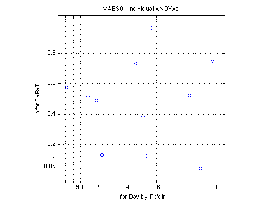
labels = D1(1).indiv_ANOVA.labels(tests_of_interest) ;

fprintf('Distribution of Fs across the %d MAES01 subjects:',N_MAES01_sbj) ;
describe(MAES01_ind_F,labels) ;
fprintf('Critical F(1,160) = %.2f (p<.05)\n',finv(.95,1,160)) ;

fprintf('\nCorresponding t values:') ;
describe(sqrt(MAES01_ind_F),labels) ;

fprintf('\nCorresponding p values:') ;
describe(MAES01_ind_p,labels) ;

fprintf('\nCorresponding PARTIAL omega^2 [%%] -- Eq.21.7 in Keppel&Wickens:') ;
describe(MAES01_ind_w2p.*100,labels) ;

fprintf('\nCorresponding COMPLETE omega^2 [%%] -- Eq.21.9') ;
describe(MAES01_ind_w2c.*100,labels) ;

DR_idx = 4 ; assert(all(labels{DR_idx}=='  DR')) ;
DRT_idx = 7 ; assert(all(labels{DRT_idx}==' DRT')) ;


%- Plot the significance values at POST vs at PRE
xtick_p = [0 .05 .1, .2:.2:1] ;

plot(MAES01_ind_p(:,DR_idx),MAES01_ind_p(:,DRT_idx),'o') ;
axis([-.05 1.05 -.05 1.05]) ; axis square ; grid on ;
set(gca,'XTick',xtick_p,'YTick',xtick_p) ;
xlabel('p for Day-by-Refdir') ;
ylabel('p for DxRxT') ;
title('MAES01 individual ANOVAs') ;

clearvars DV IVs err_idx DR_idx DRT_idx ;

% Conclusion: The Day-by-Refdir interaction is significant for 1 subject
% only (sbj355, D1(2)).  The Day-by-Refdir-by-Test interaction is
% significant for 1 other subject (sbj359, D1(5)).  The mean effect of the
% Refdir factor is not significant for anybody.
% All in all, this suggests that Refdir does not have any significant
% effects, which is evidence against the rep.modification hypothesis.
% *The question is, however, do we have enough power?*
Distribution of Fs across the 11 MAES01 subjects:
    Mean  Std.dev       Min     Q25  Median     Q75     Max
------------------------------------------------------------
  21.266   21.304      0.30    5.15   17.45   31.33   74.28     D
   1.073    0.972      0.03    0.12    1.03    1.70    3.14     R
  74.922   91.062      0.70    8.27   29.73  139.07  269.56     T
   1.300    2.147      0.00    0.12    0.43    1.58    7.41    DR
  16.399   23.305      0.01    1.90    7.12   16.22   64.48    DT
   1.006    1.199      0.01    0.07    0.32    1.93    3.62    RT
   1.045    1.344      0.00    0.16    0.42    1.92    4.22   DRT
------------------------------------------------------------
  16.716   20.190      0.15    2.26    8.07   27.68   60.96
Critical F(1,160) = 3.90 (p<.05)

Corresponding t values:
    Mean  Std.dev       Min     Q25  Median     Q75     Max
------------------------------------------------------------
   4.051    2.311      0.55    2.20    4.18    5.59    8.62     D
   0.901    0.536      0.18    0.32    1.02    1.31    1.77     R
   6.947    5.416      0.84    2.87    5.45   11.79   16.42     T
   0.876    0.766      0.04    0.32    0.66    1.26    2.72    DR
   3.178    2.632      0.11    1.36    2.67    4.02    8.03    DT
   0.808    0.623      0.08    0.26    0.56    1.39    1.90    RT
   0.838    0.614      0.04    0.39    0.65    1.36    2.06   DRT
------------------------------------------------------------
   2.514    1.843      0.26    1.10    2.17    3.82    5.93

Corresponding p values:
    Mean  Std.dev       Min     Q25  Median     Q75     Max
------------------------------------------------------------
   0.071    0.176      0.00    0.00    0.00    0.05    0.59     D
   0.426    0.290      0.08    0.19    0.31    0.75    0.86     R
   0.057    0.131      0.00    0.00    0.00    0.00    0.40     T
   0.486    0.316      0.01    0.21    0.51    0.75    0.97    DR
   0.167    0.299      0.00    0.00    0.01    0.19    0.91    DT
   0.496    0.323      0.06    0.17    0.57    0.79    0.94    RT
   0.477    0.290      0.04    0.19    0.52    0.70    0.97   DRT
------------------------------------------------------------
   0.311    0.261      0.03    0.11    0.27    0.46    0.80

Corresponding PARTIAL omega^2 [%] -- Eq.21.7 in Keppel&Wickens:
    Mean  Std.dev       Min     Q25  Median     Q75     Max
------------------------------------------------------------
   9.878    9.009      0.00    2.39    8.92   15.27   30.37     D
   0.242    0.391      0.00    0.00    0.02    0.42    1.26     R
  22.865   23.110      0.00    4.15   14.60   45.08   61.52     T
   0.449    1.092      0.00    0.00    0.00    0.34    3.68    DR
   7.325   10.003      0.00    0.53    3.51    8.30   27.42    DT
   0.292    0.493      0.00    0.00    0.00    0.55    1.54    RT
   0.315    0.609      0.00    0.00    0.00    0.58    1.88   DRT
------------------------------------------------------------
   5.909    6.387      0.00    1.01    3.86   10.08   18.24

Corresponding COMPLETE omega^2 [%] -- Eq.21.9
    Mean  Std.dev       Min     Q25  Median     Q75     Max
------------------------------------------------------------
   7.482    7.426      0.00    1.58    4.77   12.41   23.30     D
   0.181    0.311      0.00    0.00    0.01    0.33    1.00     R
  20.645   21.222      0.00    3.08   12.28   43.14   51.93     T
   0.392    1.002      0.00    0.00    0.00    0.29    3.37    DR
   4.753    6.223      0.00    0.27    3.22    6.56   20.18    DT
   0.164    0.267      0.00    0.00    0.00    0.30    0.77    RT
   0.153    0.267      0.00    0.00    0.00    0.31    0.64   DRT
------------------------------------------------------------
   4.824    5.245      0.00    0.70    2.90    9.05   14.46
151a: How many effects are significant at various alpha levels?
See Section 164 for the analogous summary of the alternative partitioning of the same variance. See Section 404 for the MAESpec02 analog. Added 2011-03-19, AAP.
alphas = [.001 .005 .01 .05 .10] ;

labels          % print column labels
MAES01_ind_p    % print the p values for each effect and each sbj

for k = 1:length(alphas)
    fprintf('p<%.3f -->  %s \n',alphas(k),mat2str(sum(MAES01_ind_p<alphas(k)))) ;
end

% We see that 8 of 11 Ss have a significant effect of Day (at p<.05).
% Also, 9 of 11 have a signif effect of Type, and 6 of 11 show DxT interaction.
%
% We will see later (Sections 260-270), however, that the grand ANOVA does
% not show a significant effect for Day.  Could it be that some subjects go
% up and other subjects go down, thus cancelling each other in the grand
% average?
labels =

    '   D'    '   R'    '   T'    '  DR'    '  DT'    '  RT'    ' DRT'


MAES01_ind_p =

    0.0000    0.7954    0.0017    0.5665    0.0000    0.2110    0.9696
    0.0018    0.8572    0.2105    0.0072    0.0084    0.9398    0.5764
    0.0009    0.6042         0    0.8166    0.2211    0.5738    0.5251
    0.0000    0.2162         0    0.4630    0.0001    0.0588    0.7346
    0.0000    0.3109         0    0.8894    0.0000    0.7313    0.0416
    0.5854    0.2848         0    0.2424    0.0817    0.1544    0.1304
    0.0000    0.0781    0.0023    0.5335    0.5634    0.5987    0.1255
    0.0000    0.8309    0.0000    0.1491    0.0506    0.1399    0.5172
    0.0627    0.1734    0.0000    0.9679    0.0031    0.8667    0.7487
    0.0000    0.1867    0.0058    0.5115    0.9089    0.3679    0.3863
    0.1315    0.3476    0.4044    0.2014    0.0002    0.8150    0.4927

p<0.001 -->  [7 0 6 0 4 0 0]
p<0.005 -->  [8 0 8 0 5 0 0]
p<0.010 -->  [8 0 9 1 6 0 0]
p<0.050 -->  [8 0 9 1 6 0 1]
p<0.100 -->  [9 1 9 1 8 1 1]
151b: How many Ss have a significant Day effect going up vs down?
See Section 405 for the MAESpec02 analog. Added 2011-03-19, AAP.
D_idx = 1 ; assert(all(labels{D_idx}=='   D')) ;

preMAE = NaN(N_MAES01_sbj,1) ;
postMAE = NaN(N_MAES01_sbj,1) ;

for k = 1:N_MAES01_sbj
    p = MAES01_ind_p(k,D_idx) ;
    preMAE(k) = round(mean(mean_MAE_by_sbj.MAES01_pretest(k,:))) ;
    postMAE(k) = round(mean(mean_MAE_by_sbj.MAES01_posttest(k,:))) ;

    fprintf('k=%2d, sbj=%d, p=%.4f, preMAE=%d, postMAE=%d: ', k,D1(k).sbj, ...
            p, preMAE(k), postMAE(k)) ;

    if (p>=.05)
        fprintf('= \n') ;    % statistically equal
    elseif (preMAE(k) < postMAE(k))
        fprintf('< \n') ;
    else
        fprintf('> \n') ;
    end
end

describe([preMAE postMAE postMAE-preMAE],{'preMAE', 'postMAE', 'MAE change'})

clearvars names tests_of_interest labels alphas D_idx p preMAE postMAE ;

% Conclusion: The overall MAE duration clearly depends on subjective
% resonse criteria.  4 of the 11 Ss showed a statistically significant
% increase at post-test relative to pre-test, 4 other Ss showed a
% significant decrease, and 3 showed insignificant change.
% This is why the grand ANOVA in Section 260 does not show signif main
% effect of Day.
k= 1, sbj=353, p=0.0000, preMAE=3039, postMAE=4950: <
k= 2, sbj=355, p=0.0018, preMAE=2379, postMAE=2858: <
k= 3, sbj=356, p=0.0009, preMAE=4601, postMAE=5420: <
k= 4, sbj=357, p=0.0000, preMAE=5981, postMAE=4652: >
k= 5, sbj=359, p=0.0000, preMAE=6959, postMAE=5838: >
k= 6, sbj=360, p=0.5854, preMAE=6910, postMAE=7020: =
k= 7, sbj=362, p=0.0000, preMAE=9097, postMAE=6490: >
k= 8, sbj=363, p=0.0000, preMAE=7180, postMAE=5594: >
k= 9, sbj=364, p=0.0627, preMAE=4199, postMAE=3475: =
k=10, sbj=366, p=0.0000, preMAE=7342, postMAE=9190: <
k=11, sbj=367, p=0.1315, preMAE=6450, postMAE=6034: =

    Mean  Std.dev       Min     Q25  Median     Q75     Max
------------------------------------------------------------
5830.636 2037.151   2379.00 4299.50 6450.00 7124.75 9097.00  preMAE
5592.818 1712.567   2858.00 4726.50 5594.00 6376.00 9190.00  postMAE
-237.818 1427.906   -2607.00 -1277.00 -416.00  734.00 1911.00  MAE change
------------------------------------------------------------
3728.545 1725.875    876.67 2583.00 3876.00 4744.92 6732.67
152: Combine the individual CI90s into a grand CI90 for MAES01
See Section 410 for the MAES02 analog
CI90 = NaN(N_MAES01_sbj,1)  ;
MS_err = NaN(N_MAES01_sbj,2) ;    % [absolute, relative_to_meanMAE]
for k = 1:N_MAES01_sbj
    CI90(k) = D1(k).indiv_ANOVA.CI90_cell_means ;
    M2 = (mean(D1(k).new_data(:,J.MAE))/msec2sec)^2 ;
    MS_err(k,:) = D1(k).indiv_ANOVA.MS_err * [1 1/M2] ;
end
mean_MAE_by_sbj.MAES01_indiv_CI90 = CI90 ;
mean_MAE_by_sbj.MAES01_grand_CI90 = sqrt(mean(CI90.^2)/N_MAES01_sbj) ;
mean_MAE_by_sbj.MAES01_MS_err = MS_err

%-- Report descriptive statistics for MS_err
describe(mean_MAE_by_sbj.MAES01_MS_err,...
         {'absolute [seconds^2]','relative to M2 for each sbj'})

clearvars CI90 MS_err M2 ;
mean_MAE_by_sbj =

     MAES01_test_type: [1 1 2 2]
        MAES01_refdir: [1 2 1 2]
     MAES01_all_cells: [11x8 double]
       MAES01_pretest: [11x4 double]
      MAES01_posttest: [11x4 double]
        MAES01_change: [11x4 double]
     MAES02_test_type: [1 1 1 1]
        MAES02_refdir: [1 2 3 4]
     MAES02_all_cells: [16x8 double]
       MAES02_pretest: [16x4 double]
      MAES02_posttest: [16x4 double]
        MAES02_change: [16x4 double]
    MAES01_indiv_CI90: [11x1 double]
    MAES01_grand_CI90: 0.2233
        MAES01_MS_err: [11x2 double]


    Mean  Std.dev       Min     Q25  Median     Q75     Max
------------------------------------------------------------
   3.874    2.537      0.96    2.19    3.16    5.58    8.33  absolute [seconds^2]
   0.130    0.103      0.04    0.08    0.10    0.13    0.43  relative to M2 for each sbj
------------------------------------------------------------
   2.002    1.320      0.50    1.13    1.63    2.85    4.38
155: Introduce the Simple effect of Refdir at Day=POSTTEST
We'll show that the conventional decomposition of the SS's in terms of the mean effect of Refdir and the DxR interaction is not the optimal way of addressing our research question about the representation modification hypothesis. There is a better way, which can detect an effect of half the size with the same statistical power.
The key idea is that the rep.modif hypothesis predicts a change in only one of the 4 cells of the DxR interaction -- the TRAIN direction at POSTTEST. At pretest, both directions are on an equal footing beacause there has been no differential practice yet. (They are also counterbalanced between subjects and are nearly symmetrical w.r.t vertical.)
% Notation: Let us label the four cells as follows:
%  * Tr1 -- TRAIN direction at PRETEST -- assume MAE=M
%  * Or1 -- TRANSF (or Ortho) direction at PRETEST -- also MAE=M by symmetry
%  * Or2 -- TRANSF at POSTTEST -- no change, assuming learning was specific
%  * Tr2 -- TRAIN at POSTTEST -- *Change expected here!*
% Let's denote by C the *relative* size of the change (increase or decrease).
% Thus, the predicted MAE for TRAIN at POSTTEST is (1+C)*M, where M is the
% (mean of the) MAE in the other 3 cells.  We'll do power analysis for a
% range of values C for the hypothetical change.

hyp_change = [.05 .10 .15 .20 .25 .30] ;  % relative to mean(MAE)

% Inspired by the example illustrated in Figure 12.3 in KeppelWickens04
% (p. 255, continued in Table 13.8 on p.283), it is perhaps easier to think
% about all this in terms of a one-way analysis with 4 levels:
%   DxR Cell          Tr1    Or1    Tr2    Or2  | Mean
% ----------------------------------------------+------
% 1 Day main effect    -1     -1     +1     +1  |  0
% 2 Refdir main eff    +1     -1     +1     -1  |  0
% 3 DxR interaction    +1     -1     -1     +1  |  0   % Eq.11.13.alt, p.227
% ----------------------------------------------+------
%
% Our hypothetical expected means will yield the following under the
% above "conventional partition":
%   DxR Cell          Tr1    Or1    Tr2    Or2  | Mean
% ----------------------------------------------+------
% 1 Day main effect    -M     -M  +(1+C)M   +M  | +C*M/4 + criterion-related changes
% 2 Refdir main eff    +M     -M  +(1+C)M   -M  | +C*M/4
% 3 DxR interaction    +M     -M  -(1+C)M   +M  | -C*M/4
% ----------------------------------------------+------
%
% We see that the conventional partition smears the change across all three
% effects being tested.  The main effect of Day is also expected to change
% due to criterion shifts, which may well dwarf the C*M term of interest
% here.  So, let's not tinker with the mean effect of Day.
%
% However, we can replace the (R + DxR) conditions with another set of
% contrasts. Note that they are still mutually orthogonal:
%   DxR Cell          Tr1    Or1    Tr2    Or2  | Mean
% ----------------------------------------------+------
% 1 Day main effect    -1     -1     +1     +1  |  0   % same as above
% 4 Refdir at PRETEST  +2     -2      0      0  |  0
% 5 Refdir at POSTTEST  0      0     +2     -2  |  0
% ----------------------------------------------+------
%
% Predicted MAE durations under the rep.modif hypothesis:
%   DxR Cell          Tr1    Or1    Tr2    Or2  | Mean
% ----------------------------------------------+------
% 1 Day main effect    -M     -M  +(1+C)M   +M  | +C*M/4 + criterion-related changes
% 4 Refdir at PRETEST +2M    -2M      0      0  |  0
% 5 Refdir at POSTTEST  0      0 +2(1+C)M  -2M  | +C*M/2
% ----------------------------------------------+------
%
% We see that the C*M term is now concentrated in line 5 only (at POSTTEST)
% rather than being split b/n lines 2 and 3 (as it was in the conventional
% partition).  This focues twice as much statistical power at detecting it.
% Section 165 below verifies that for the actual numbers in our study.
%
% These contrasts should be crossed with the Test_type factor, but we
% aren't going to bother with this here because SS(R_at_PRExT)+SS(R_at_POSTxT)
% is equal (and hence bounded by) SS(DxRxT) which was (barely) significant
% for a single subject only.

% Technical note: The formulas normalize by the sum of squared contrast coefs,
% so the tables above should have used [+1/2 -1/2 -1/2 +1/2] for DxR and
% [0 0 +1/sqrt2 -1/sqrt2] for R_at_POSTTEST (henceforth abbreviated "Rat1").
% The contrast coefs will be represented as column vectors of length 8 that
% operate on the row vector of cell means across the 8 conditions.

% See Section 500 below for the contrasts for the MAESpec02 experiment.
157: MAES01 cell_nanmean indices: V1
    index: [1 2 3 4 5 6 7 8]
      day: [1 1 1 1 2 2 2 2]
test_type: [1 1 2 2 1 1 2 2]
   refdir: [1 2 1 2 1 2 1 2]
%- Unconditional indices for all 3 factors V1.pretest = (D1(1).day==enum.PRETEST) ; % [1 1 1 1 0 0 0 0] V1.posttest = (D1(1).day==enum.POSTTEST) ; % [0 0 0 0 1 1 1 1] V1.static = (D1(1).test_type==enum.STATIC) ; % [1 1 0 0 1 1 0 0] V1.dynamic = (D1(1).test_type==enum.DYNAMIC) ; % [0 0 1 1 0 0 1 1] V1.train = (D1(1).refdir==enum.TRAIN) ; % [1 0 1 0 1 0 1 0] V1.transf = (D1(1).refdir==enum.TRANSF) ; % [0 1 0 1 0 1 0 1] %- Conditional indices for the Refdir factor V1.train4T = V1.train(V1.static) ; % [1 0 1 0] % when Test_type is fixed V1.transf4T = V1.transf(V1.static) ; % [0 1 0 1] V1.train4D = V1.train(V1.pretest) ; % [1 0 1 0] % when Day is fixed V1.transf4D = V1.transf(V1.pretest) ; % [0 1 0 1] %- Conditional indices for the Day factor V1.pretest4T = V1.pretest(V1.static) ; % [1 1 0 0] % when Test_type is fixed V1.posttest4T = V1.posttest(V1.static) ; % [0 0 1 1] V1.pretest4R = V1.pretest(V1.train) ; % [1 1 0 0] % when Refdir is fixed V1.posttest4R = V1.posttest(V1.transf) ; % [0 0 1 1] %- Conditional indices for the Test_type factor V1.static4D = V1.static(V1.pretest) ; % [1 1 0 0] % when Day is fixed V1.dynamic4D = V1.dynamic(V1.pretest) ; % [0 0 1 1] V1.static4R = V1.static(V1.train) ; % [1 0 1 0] % when Refdir is fixed V1.dynamic4R = V1.dynamic(V1.train) % [0 1 0 1]
V1 =

       pretest: [1 1 1 1 0 0 0 0]
      posttest: [0 0 0 0 1 1 1 1]
        static: [1 1 0 0 1 1 0 0]
       dynamic: [0 0 1 1 0 0 1 1]
         train: [1 0 1 0 1 0 1 0]
        transf: [0 1 0 1 0 1 0 1]
       train4T: [1 0 1 0]
      transf4T: [0 1 0 1]
       train4D: [1 0 1 0]
      transf4D: [0 1 0 1]
     pretest4T: [1 1 0 0]
    posttest4T: [0 0 1 1]
     pretest4R: [1 1 0 0]
    posttest4R: [0 0 1 1]
      static4D: [1 1 0 0]
     dynamic4D: [0 0 1 1]
      static4R: [1 0 1 0]
     dynamic4R: [0 1 0 1]
160: Define contrast coefficients
contrasts1 = NaN(N_cells,5) ;
contrast_names1 = cell(1,5) ;

% 1 Day main effect    -1     -1     +1     +1  |  0
%   DxR Cell          Tr1    Or1    Tr2    Or2  | Mean
V1.Day = 1 ;
contrast_names1{V1.Day} = 'Day' ;
contrasts1(V1.pretest,V1.Day) = -1 ;
contrasts1(V1.posttest,V1.Day) = +1 ;

% 2 Refdir main eff    +1     -1     +1     -1  |  0
%   DxR Cell          Tr1    Or1    Tr2    Or2  | Mean
V1.Refdir = 2 ;
contrast_names1{V1.Refdir} = 'Refdir' ;
contrasts1(V1.train,V1.Refdir) = +1 ;
contrasts1(V1.transf,V1.Refdir) = -1 ;

% 3 DxR interaction    +1     -1     -1     +1  |  0   % Eq.11.13.alt, p.227
%   DxR Cell          Tr1    Or1    Tr2    Or2  | Mean
V1.DxR = 3 ;
contrast_names1{V1.DxR} = 'DxR' ;
contrasts1(V1.pretest&V1.train,V1.DxR) = +1 ;
contrasts1(V1.pretest&V1.transf,V1.DxR) = -1 ;
contrasts1(V1.posttest&V1.train,V1.DxR) = -1 ;
contrasts1(V1.posttest&V1.transf,V1.DxR) = +1 ;

% 4 Refdir at PRETEST  +2     -2      0      0  |  0
%   DxR Cell          Tr1    Or1    Tr2    Or2  | Mean
V1.R_at_PRE = 4 ;
contrast_names1{V1.R_at_PRE} = 'R_at_PRE' ;
contrasts1(V1.pretest&V1.train,V1.R_at_PRE) = +1 ;
contrasts1(V1.pretest&V1.transf,V1.R_at_PRE) = -1 ;
contrasts1(V1.posttest,V1.R_at_PRE) = 0 ;

% 5 Refdir at POSTTEST  0      0     +2     -2  |  0
%   DxR Cell          Tr1    Or1    Tr2    Or2  | Mean
V1.R_at_POST = 5 ;
contrast_names1{V1.R_at_POST} = 'R_at_POST' ;
contrasts1(V1.posttest&V1.train,V1.R_at_POST) = +1 ;
contrasts1(V1.posttest&V1.transf,V1.R_at_POST) = -1 ;
contrasts1(V1.pretest,V1.R_at_POST) = 0 ;

% R_at_PRE_by_T and R_at_POST_by_T can be defined here if necessary.

% Display the contrast names (and the coefs below)
contrast_names1

% Normalize to unit length
normalize_coefs = @(c) (c ./ repmat(sqrt(sum(c.^2)),size(c,1),1)) ;
contrasts1 = normalize_coefs(contrasts1)
contrast_names1 =

    'Day'    'Refdir'    'DxR'    'R_at_PRE'    'R_at_POST'


contrasts1 =

   -0.3536    0.3536    0.3536    0.5000         0
   -0.3536   -0.3536   -0.3536   -0.5000         0
   -0.3536    0.3536    0.3536    0.5000         0
   -0.3536   -0.3536   -0.3536   -0.5000         0
    0.3536    0.3536   -0.3536         0    0.5000
    0.3536   -0.3536    0.3536         0   -0.5000
    0.3536    0.3536   -0.3536         0    0.5000
    0.3536   -0.3536    0.3536         0   -0.5000
162: Calculate SS for the Contrasts
Equation 4.5 in Keppel & Wickens (2004, p. 69). Also MS==SS because df=1.
Each contrast is calculated twice. First from the complete MAE (with imputed missing values) -- as a sanity check with the ANOVA SS that too are calculated on the complete MAE. Second from the MAE_duration (with NaNs) -- free of imputation assumptions. All subsequent analyses use the second (nanmean) set of contrasts.
See Section 520 for the MAESpec02 analog.
eq0 = @(x) (max(abs(x))<1e-8) ;   % equality check with tolerance

MAES01_psy_F = NaN(N_MAES01_sbj,length(contrast_names1)) ;
MAES01_psy_p = NaN(N_MAES01_sbj,length(contrast_names1)) ;
MAES01_psy_w2p = NaN(N_MAES01_sbj,length(contrast_names1)) ;
MAES01_psy_w2c = NaN(N_MAES01_sbj,length(contrast_names1)) ;

for k = 1:N_MAES01_sbj
    %- Retrieve the cell means of the original design
    M = D1(k).cell_nanmean_MAE ./ msec2sec ; % [N_cells x 1], w/ NaNs
    M0 = mean(D1(k).MAE) ./ msec2sec ;       % [N_cells x 1], no missing vals

    %- Augment the indiv_ANOVA structure
    st = D1(k).indiv_ANOVA ;
    st.contrast_names = contrast_names1 ;

    %- Calculate the "observed value psy_hat of each contrast"
    psy = M*contrasts1 ;       % [1x5], Eq.4.4
    psy0 = M0*contrasts1 ;     % [1x5], Eq.4.4
    st.psy_NaN = psy ;
    st.psy_noNaN = psy0 ;

    %- Convert each observed contrast into a sum of squares (Eq.4.5)
    % Note that the coefficients are already normalized.
    SS = N_reps_per_cell * psy.^2 ;
    SS0 = N_reps_per_cell * psy0.^2 ;
    st.SS_psy_NaN = SS ;
    st.SS_psy_noNaN = SS0 ;

    %- Sanity check: SS0(V1.Day) should match indiv_ANOVA.SS('D'=1)
    assert(eq0(SS0(V1.Day) - st.SS(1))) ;

    %- Sanity check: SS0(V1.Refdir) should match indiv_ANOVA.SS('R'=2)
    assert(eq0(SS0(V1.Refdir) - st.SS(2))) ;

    %- Sanity check: SS0(V1.DxR) should match indiv_ANOVA.SS('DR'=4)
    assert(eq0(SS0(V1.DxR) - st.SS(4))) ;

    %- Sanity check: Additivity of conventional and new partition
    assert(eq0((SS0(V1.Refdir)+SS0(V1.DxR)) - ...       % w/o NaNs
               (SS0(V1.R_at_PRE)+SS0(V1.R_at_POST)) )) ;
    assert(eq0((SS(V1.Refdir)+SS(V1.DxR)) - ...         % w/  NaNs
               (SS(V1.R_at_PRE)+SS(V1.R_at_POST)) )) ;

    %- Calculate F ratios
    % All these contrasts have df=1 and hence MS=SS. All use a common
    % error term -- MS_err from the overall analysis (Eq 4.6).
    F = SS ./ st.MS_err ;
    F0 = SS0 ./ st.MS_err ;
    st.F_psy_NaN = F ;
    st.t_psy_NaN = sqrt(F) ;
    st.F_psy_noNaN = F0 ;
    st.t_psy_noNaN = sqrt(F0) ;
    MAES01_psy_F(k,:) = F ;

    %- Calculate significance
    st.p_psy_NaN = 1-fcdf(F,1,st.adjusted_df_err) ;
    st.p_psy_noNaN = 1-fcdf(F0,1,st.adjusted_df_err) ;
    MAES01_psy_p(k,:) = st.p_psy_noNaN ;

    %- Calculate partial and complete omega-squared (Eqs. 21.7 & 21.8)
    N = st.df(end)+1 ;  % 168 = total # of scores
    w2 = 1 .* (F-1) ;   % df=1
    w2 = max(0,w2) ;  % F values < 1.0 are entirely due to sampling error.
    st.partial_omega2_psy = w2./(w2+N) ;        % Eq. 21.7
    st.complete_omega2_psy = w2./(sum(w2)+N) ;  % Eq. 21.9
    MAES01_psy_w2p(k,:) = st.partial_omega2_psy ;
    MAES01_psy_w2c(k,:) = st.complete_omega2_psy ;

    %- Store and move on
    D1(k).indiv_ANOVA = st ;
end
clearvars k M M0 st psy psy0 SS SS0 F F0 w2 N ;


%- Print a representative individual ANOVA.
%  This subject (#353) had 1 missing value and therefore
%  the adjusted_df_err is 1 less than df(err_idx)
fprintf('Representative individual ANOVA for sbj #%d\n',D1(1).sbj) ;
D1(1).indiv_ANOVA

% The critical value for a linear contrast with df_err=160, p<.05, is:
fprintf('F(.95,1,160) = %.3f \n',finv(.95,1,160))
Representative individual ANOVA for sbj #353

ans =

                    lbl: [9x4 char]
                 labels: {'   D'  '   R'  '   T'  '  DR'  '  DT'  '  RT'  ' DRT'  ' err'  'Totl'}
                     SS: [155.7067 0.1414 21.3505 0.6918 135.1610 3.3059 0.0031 335.3822 651.7425]
                     df: [1 1 1 1 1 1 1 160 167]
                     MS: [155.7067 0.1414 21.3505 0.6918 135.1610 3.3059 0.0031 2.0961 3.9026]
                 MS_err: 2.0961
     std_err_cell_means: 0.3159
        CI90_cell_means: 0.5449
        adjusted_df_err: 159
                      F: [74.2826 0.0675 10.1856 0.3300 64.4810 1.5771 0.0015]
                      t: [8.6187 0.2598 3.1915 0.5745 8.0300 1.2558 0.0382]
                      p: [6.4393e-15 0.7954 0.0017 0.5665 2.0439e-13 0.2110 0.9696]
         partial_omega2: [0.3037 0 0.0518 0 0.2742 0.0034 0]
        complete_omega2: [0.2330 0 0.0292 0 0.2018 0.0018 0]
         contrast_names: {'Day'  'Refdir'  'DxR'  'R_at_PRE'  'R_at_POST'}
                psy_NaN: [2.7017 -0.0608 0.1602 0.0703 -0.1563]
              psy_noNaN: [2.7230 -0.0821 0.1815 0.0703 -0.1864]
             SS_psy_NaN: [153.2826 0.0776 0.5391 0.1038 0.5129]
           SS_psy_noNaN: [155.7067 0.1414 0.6918 0.1038 0.7294]
              F_psy_NaN: [73.1262 0.0370 0.2572 0.0495 0.2447]
              t_psy_NaN: [8.5514 0.1924 0.5071 0.2225 0.4946]
            F_psy_noNaN: [74.2826 0.0675 0.3300 0.0495 0.3480]
            t_psy_noNaN: [8.6187 0.2598 0.5745 0.2225 0.5899]
              p_psy_NaN: [9.5479e-15 0.8477 0.6128 0.8242 0.6215]
            p_psy_noNaN: [6.4393e-15 0.7954 0.5665 0.8242 0.5561]
     partial_omega2_psy: [0.3004 0 0 0 0]
    complete_omega2_psy: [0.3004 0 0 0 0]

F(.95,1,160) = 3.900
163: Report the contrast-based test results
Note: The F ratios for Day, Refdir, and DxR are based on nanmeans and hence differ slightly from the ones reported in section 151 above. Arguably, the ones reported here should take precedence because they do not depend on assumptions about filled-in missing values. In this scheme, the imputed values only influence the MS_err (but not adjusted_df_err). (Caveat: The significance may have dropped a little because we got rid of the imputed missing values.)
See Section 530 for the MAESpec02 analog.
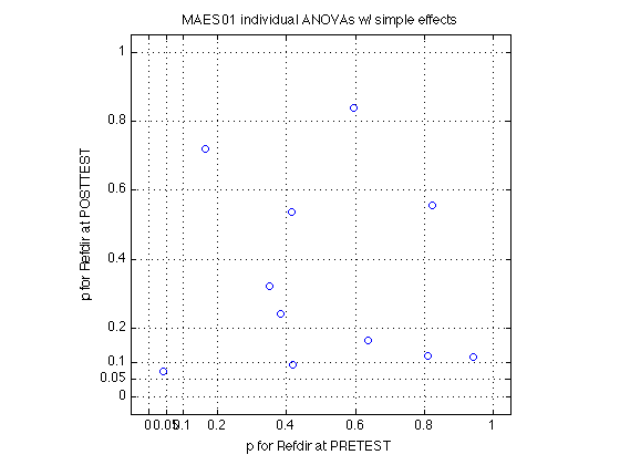
MAES01_psy_F
disp(contrast_names1)

fprintf('Distribution of contrast-based Fs, %d MAES01 Ss:',N_MAES01_sbj) ;
describe(MAES01_psy_F,contrast_names1) ;
fprintf('Critical F(1,160) = %.2f (p<.05)\n',finv(.95,1,160)) ;

fprintf('\nCorresponding t values:') ;
describe(sqrt(MAES01_psy_F),contrast_names1) ;

fprintf('\nCorresponding p values:') ;
describe(MAES01_psy_p,contrast_names1) ;

fprintf('\nCorresponding PARTIAL omega^2 [%%] -- Eq.21.7 in Keppel&Wickens:') ;
describe(MAES01_psy_w2p.*100,contrast_names1) ;

fprintf('\nCorresponding COMPLETE omega^2 [%%] -- Eq.21.9') ;
describe(MAES01_psy_w2c.*100,contrast_names1) ;

%- Plot p(R_at_POST) vs p(R_at_PRE)
plot(MAES01_psy_p(:,V1.R_at_PRE),MAES01_psy_p(:,V1.R_at_POST),'o') ;
axis([-.05 1.05 -.05 1.05]) ; axis square ; grid on ;
set(gca,'XTick',xtick_p,'YTick',xtick_p) ;
xlabel('p for Refdir at PRETEST') ;
ylabel('p for Refdir at POSTTEST') ;
title('MAES01 individual ANOVAs w/ simple effects') ;

% Conclusion: *none* of the 11 Ss show a significant effect for R_at_POST!
% We applied a *more powerful* test and got less sifnificant results!!
% Only sbj355 [D1(2)] shows (barely) significant R_at_PRETEST effect.
% The POSTTEST tends to yield lower p values (closer to significance) than
% the PRETEST, which can be interpreted as a very tentative trend in the
% direction predicted by the rep.modif hypothesis.
% All in all, however, the preponderance of the evidence is against it.
% The question still stands: *Do we have enough power to assert the null?*
MAES01_psy_F =

   73.1262    0.0370    0.2572    0.0495    0.2447
   10.0673    0.0325    7.4110    4.2124    3.2312
   11.4987    0.2697    0.0540    0.2825    0.0412
   26.4518    1.5997    0.5759    2.0477    0.1280
   15.0396    0.8676    0.0526    0.6738    0.2464
    0.2987    1.1519    1.3770    0.0050    2.5239
   35.1007    2.9363    0.4673    0.5304    2.8732
   33.0332    0.0457    2.1017    0.7637    1.3838
    3.5133    1.8695    0.0016    0.8805    0.9906
   17.2161    1.6861    0.3971    0.2233    1.8599
    2.2979    0.8873    1.6460    0.0581    2.4752

    'Day'    'Refdir'    'DxR'    'R_at_PRE'    'R_at_POST'

Distribution of contrast-based Fs, 11 MAES01 Ss:
    Mean  Std.dev       Min     Q25  Median     Q75     Max
------------------------------------------------------------
  20.695   21.055      0.30    5.15   15.04   31.39   73.13  Day
   1.035    0.932      0.03    0.10    0.89    1.66    2.94  Refdir
   1.304    2.145      0.00    0.10    0.47    1.58    7.41  DxR
   0.884    1.248      0.01    0.10    0.53    0.85    4.21  R_at_PRE
   1.454    1.201      0.04    0.25    1.38    2.51    3.23  R_at_POST
------------------------------------------------------------
   5.074    5.316      0.08    1.14    3.66    7.60   18.18
Critical F(1,160) = 3.90 (p<.05)

Corresponding t values:
    Mean  Std.dev       Min     Q25  Median     Q75     Max
------------------------------------------------------------
   3.990    2.291      0.55    2.20    3.88    5.60    8.55  Day
   0.882    0.533      0.18    0.29    0.94    1.29    1.71  Refdir
   0.883    0.760      0.04    0.30    0.68    1.26    2.72  DxR
   0.762    0.578      0.07    0.30    0.73    0.92    2.05  R_at_PRE
   1.067    0.589      0.20    0.50    1.18    1.58    1.80  R_at_POST
------------------------------------------------------------
   1.517    0.950      0.21    0.72    1.48    2.13    3.37

Corresponding p values:
    Mean  Std.dev       Min     Q25  Median     Q75     Max
------------------------------------------------------------
   0.071    0.176      0.00    0.00    0.00    0.05    0.59  Day
   0.426    0.290      0.08    0.19    0.31    0.75    0.86  Refdir
   0.486    0.316      0.01    0.21    0.51    0.75    0.97  DxR
   0.507    0.283      0.04    0.36    0.42    0.77    0.94  R_at_PRE
   0.343    0.275      0.07    0.11    0.24    0.55    0.84  R_at_POST
------------------------------------------------------------
   0.367    0.268      0.04    0.18    0.30    0.57    0.84

Corresponding PARTIAL omega^2 [%] -- Eq.21.7 in Keppel&Wickens:
    Mean  Std.dev       Min     Q25  Median     Q75     Max
------------------------------------------------------------
   9.622    8.937      0.00    2.39    7.71   15.30   30.04  Day
   0.228    0.359      0.00    0.00    0.00    0.39    1.14  Refdir
   0.449    1.092      0.00    0.00    0.00    0.34    3.68  DxR
   0.227    0.578      0.00    0.00    0.00    0.00    1.88  R_at_PRE
   0.447    0.511      0.00    0.00    0.23    0.89    1.31  R_at_POST
------------------------------------------------------------
   2.194    2.295      0.00    0.48    1.59    3.39    7.61

Corresponding COMPLETE omega^2 [%] -- Eq.21.9
    Mean  Std.dev       Min     Q25  Median     Q75     Max
------------------------------------------------------------
   9.535    8.918      0.00    2.30    7.71   15.18   30.04  Day
   0.201    0.306      0.00    0.00    0.00    0.35    0.94  Refdir
   0.413    1.007      0.00    0.00    0.00    0.34    3.39  DxR
   0.203    0.522      0.00    0.00    0.00    0.00    1.70  R_at_PRE
   0.409    0.466      0.00    0.00    0.19    0.89    1.18  R_at_POST
------------------------------------------------------------
   2.152    2.244      0.00    0.46    1.58    3.35    7.45
164: How many effects are significant at various alpha levels?
See Section 151a for the analogous summary of the conventional partitioning of the same variance. See Section 531 for the MAESpec02 analog. Added 2011-03-19, AAP.
alphas = [.001 .005 .01 .05 .10] ;

contrast_names1     % print column labels
MAES01_psy_F        % print the F statistics for each effect and each sbj
MAES01_psy_p        % print the p values for each effect and each sbj

for k = 1:length(alphas)
    fprintf('p<%.3f -->  %s \n',alphas(k),mat2str(sum(MAES01_psy_p<alphas(k)))) ;
end

% We verify the result from Section 151a that that 8 of 11 Ss have a
% significant effect of Day (at p<.05) and that 0 out of 11 have a
% significant effect of Refdir.  The new aspect concerns the simple effects:
%
% 1 of 11 Ss shows a (barely, p<.042) significant simple effect of Refdir
% at PRETEST.  This is, undoubtedly, a Type I error because the two
% directions are equivalent at pretest because no training has occurred
% yet.  This is a nice validation of this symmetry (and of the danger of
% Type I errors with repeated tests.)
%
% The main result is, to repeat, that 0 of 11 show Refdir at POSTTEST.

clearvars k alphas ;
contrast_names1 =

    'Day'    'Refdir'    'DxR'    'R_at_PRE'    'R_at_POST'


MAES01_psy_F =

   73.1262    0.0370    0.2572    0.0495    0.2447
   10.0673    0.0325    7.4110    4.2124    3.2312
   11.4987    0.2697    0.0540    0.2825    0.0412
   26.4518    1.5997    0.5759    2.0477    0.1280
   15.0396    0.8676    0.0526    0.6738    0.2464
    0.2987    1.1519    1.3770    0.0050    2.5239
   35.1007    2.9363    0.4673    0.5304    2.8732
   33.0332    0.0457    2.1017    0.7637    1.3838
    3.5133    1.8695    0.0016    0.8805    0.9906
   17.2161    1.6861    0.3971    0.2233    1.8599
    2.2979    0.8873    1.6460    0.0581    2.4752


MAES01_psy_p =

    0.0000    0.7954    0.5665    0.8242    0.5561
    0.0018    0.8572    0.0072    0.0418    0.0741
    0.0009    0.6042    0.8166    0.5958    0.8394
    0.0000    0.2162    0.4630    0.1640    0.7210
    0.0000    0.3109    0.8894    0.4150    0.5358
    0.5854    0.2848    0.2424    0.9436    0.1141
    0.0000    0.0781    0.5335    0.4178    0.0920
    0.0000    0.8309    0.1491    0.3835    0.2412
    0.0627    0.1734    0.9679    0.3495    0.3211
    0.0000    0.1867    0.5115    0.6372    0.1626
    0.1315    0.3476    0.2014    0.8098    0.1176

p<0.001 -->  [7 0 0 0 0]
p<0.005 -->  [8 0 0 0 0]
p<0.010 -->  [8 0 1 0 0]
p<0.050 -->  [8 0 1 1 0]
p<0.100 -->  [9 1 1 1 2]
165: Power analysis for the individual MAES01 ANOVAs
We follow the great presentation in Sections 8.4, 8.5, 11.7 and 13.5 in Keppel & Wickens (2004).
The power to reject the null hypothesis (all means=gradmean) must be calculated with respect to a concrete alternative hypothesis. This is where the frequentist framework acquires a Bayesian flavor.
Our alternative hyp is specified as a one-parameter family, as described in Section 155 above. The parameter in question is the hypothesized change in the MAE duration for the trained direction at posttest, relative (that is, divided by) the average MAE. We're going to calculate the power for the values in HYP_CHANGE.
See Section 550 for the MAESpec02 analog.
pwr1.contrast_names = contrast_names1 ;
pwr1.contrasts = contrasts1 ;
pwr1.hyp_change = hyp_change ;      % [1x6]
N_hyp_change = length(hyp_change) ;

%- Postulate population means for each of these 6 alternative hypotheses
hyp_MAE_means = NaN(N_hyp_change,N_cells) ;    % [6x8]

hyp_MAE_means(:,V1.pretest) = 1 ;              % = mean MAE
hyp_MAE_means(:,V1.posttest&V1.transf) = 1 ;
hyp_MAE_means(:,V1.posttest&V1.train) = ...
    repmat(1+hyp_change',1,sum(V1.posttest&V1.train))
pwr1.hyp_MAE_means = hyp_MAE_means ;

%- Calculate the hypothesized contrast values (Eq. 4.4)
hyp_psy = hyp_MAE_means * contrasts1        % [6x5] = [6x8]*[8x5]
pwr1.hyp_psy = hyp_psy ;

%- Calculate the variance sigma^2_psy for each contrast (Eq.8.13)
% (The coefficients are already normalized.)
hyp_s2_psy = (hyp_psy.^2)'/2
pwr1.hyp_s2_psy = hyp_s2_psy ;

%- Take the median, normalized MS_err calculated in Section 152 above:
pwr1.median_norm_MS_err = median(mean_MAE_by_sbj.MAES01_MS_err(:,2)) ;

%- Calculate the partial effect size (omega^2) for each contrast (Eq.8.15)
% Notice how the R_at_POST aggregates the effects of Refdir and DxR at the
% expense of R_at_PRE, in exact agreement with our theoretical motivation
% in Section 155 above.   This is precisely why we introduced contrasts
% in the first place. It's payback time now :)
w2p = pwr1.hyp_s2_psy ./ (pwr1.hyp_s2_psy+pwr1.median_norm_MS_err)
pwr1.partial_omega2 = w2p ;

%- Calculate the "noncentrality parameter phi" (Eq. 8.19)
phi = sqrt((N_reps_per_cell.*w2p)./(1-w2p))
pwr1.phi = phi ;

clearvars N_hyp_change hyp_MAE_means hyp_psy hyp_s2_psy w2p phi ;
hyp_MAE_means =

    1.0000    1.0000    1.0000    1.0000    1.0500    1.0000    1.0500    1.0000
    1.0000    1.0000    1.0000    1.0000    1.1000    1.0000    1.1000    1.0000
    1.0000    1.0000    1.0000    1.0000    1.1500    1.0000    1.1500    1.0000
    1.0000    1.0000    1.0000    1.0000    1.2000    1.0000    1.2000    1.0000
    1.0000    1.0000    1.0000    1.0000    1.2500    1.0000    1.2500    1.0000
    1.0000    1.0000    1.0000    1.0000    1.3000    1.0000    1.3000    1.0000


hyp_psy =

    0.0354    0.0354   -0.0354         0    0.0500
    0.0707    0.0707   -0.0707         0    0.1000
    0.1061    0.1061   -0.1061         0    0.1500
    0.1414    0.1414   -0.1414         0    0.2000
    0.1768    0.1768   -0.1768         0    0.2500
    0.2121    0.2121   -0.2121         0    0.3000


hyp_s2_psy =

    0.0006    0.0025    0.0056    0.0100    0.0156    0.0225
    0.0006    0.0025    0.0056    0.0100    0.0156    0.0225
    0.0006    0.0025    0.0056    0.0100    0.0156    0.0225
         0         0         0         0         0         0
    0.0013    0.0050    0.0112    0.0200    0.0312    0.0450


w2p =

    0.0063    0.0246    0.0536    0.0915    0.1360    0.1848
    0.0063    0.0246    0.0536    0.0915    0.1360    0.1848
    0.0063    0.0246    0.0536    0.0915    0.1360    0.1848
         0         0         0         0         0         0
    0.0124    0.0480    0.1018    0.1677    0.2395    0.3120


phi =

    0.3637    0.7274    1.0910    1.4547    1.8184    2.1821
    0.3637    0.7274    1.0910    1.4547    1.8184    2.1821
    0.3637    0.7274    1.0910    1.4547    1.8184    2.1821
         0         0         0         0         0         0
    0.5143    1.0286    1.5430    2.0573    2.5716    3.0859
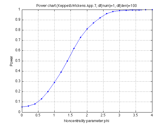
166: Power chart in Appendix A.7 (Keppel & Wickens, 2004)
We use the nomogram for df(num)=1 on p. 590 as all contrasts have df=1. We interpolate between the lines for df(den)=100 and df(den)=Inf as our MS_err has df=160. (These two lines practically overlap in our region.)
We reproduce this line of the nomogram here, and then use interp1: Use like this: interp1(power_chart.phi,power_chart.power,my_phi)
power_chart.name = 'Appendix A.7 in Keppel & Wickens (2004)' ;
power_chart.df_numerator = 1 ;
power_chart.df_denominator = 100 ;
power_chart.phi   = [  0  .2  .4  .6  .8 1.0, 1.2 1.4 1.6 1.8 2.0, ...
                         2.2 2.4 2.6 2.8 3.0, 3.2  3.4  3.6  3.8  4.0] ;
power_chart.power = [.05 .06 .08 .13 .20 .29, .39 .50 .62 .73 .81, ...
                         .87 .92 .96 .98 .99,.993 .996 .997 .998 .999] ;

plot(power_chart.phi,power_chart.power,'.-') ;
xlabel('Noncentrality parameter phi') ;
ylabel('Power') ;
axis([0 4 0 1]) ; grid on ;
title('Power chart (Keppel&Wickens App.7, df(num)=1, df(den)=100') ;
168: Power analysis, continued
power = interp1(power_chart.phi,power_chart.power,pwr1.phi)
pwr1.power = power ;

%- Pull out the two most relevant tests
pwr1.power_DxR = power(V1.DxR,:) ;
pwr1.power_R_at_POST = power(V1.R_at_POST,:) ;

clearvars power ;
power =

    0.0764    0.1746    0.3355    0.5328    0.7374    0.8646
    0.0764    0.1746    0.3355    0.5328    0.7374    0.8646
    0.0764    0.1746    0.3355    0.5328    0.7374    0.8646
    0.0500    0.0500    0.0500    0.0500    0.0500    0.0500
    0.1086    0.3043    0.5858    0.8272    0.9543    0.9913
170: Family-wise power across the 11 individual MAES01 tests
See Section 580 for the MAESpec02 analog.
The above power is for each individual test. Admittedly, the power is low for the small effect sizes. But we have 11 independent subjects and none of them turned out significant for the Refdir_at_POST test. We can calculate the probability of that outcome under each hypothesis:
p_0ofN = @(p,N) ((1-p).^N) ;
p_1ofN = @(p,N) (N.*p.*(1-p).^(N-1)) ;

pwr1.comment_0of11 = 'When the outcome is 0 hits out of 11 individual tests' ;
pwr1.prob_0of11_DxR = p_0ofN(pwr1.power_DxR,N_MAES01_sbj) ;
pwr1.prob_0of11_R_at_POST = p_0ofN(pwr1.power_R_at_POST,N_MAES01_sbj) ;

%- Probability of making 0 type-I errors in 11 tests if the null hyp is true
pwr1.prob_0of11_null = p_0ofN(.05,N_MAES01_sbj) ;    % 0.5688

%- Bayes factor null/alt, given 0 of 11 tests turn out significant
pwr1.BF_0of11_DxR = pwr1.prob_0of11_null ./ pwr1.prob_0of11_DxR ;
pwr1.BF_0of11_R_at_POST = pwr1.prob_0of11_null ./ pwr1.prob_0of11_R_at_POST ;

%- What about 1 signif outcome out of 11:  N*p*(1-p)^(N-1)
pwr1.comment_1of11 = 'When the outcome is 1 hits out of 11 individual tests' ;
pwr1.prob_1of11_DxR = p_1ofN(pwr1.power_DxR,N_MAES01_sbj) ;
pwr1.prob_1of11_R_at_POST = p_1ofN(pwr1.power_R_at_POST,N_MAES01_sbj) ;
pwr1.prob_1of11_null = p_1ofN(.05,N_MAES01_sbj) ; % 0.3293

%- Bayes factor null/alt, given 1 of 11 tests turn out significant
pwr1.BF_1of11_DxR = pwr1.prob_1of11_null ./ pwr1.prob_1of11_DxR ;
pwr1.BF_1of11_R_at_POST = pwr1.prob_1of11_null ./ pwr1.prob_1of11_R_at_POST

% Conclusion: We do have power to assert that the relative MAE change at
% posttest is less than 10%, with p<.0185  [see prob_0of11_R_at_POST(2)].
% It is 30.7928 times more likely to observe our outcome (0 of 11) under
% no MAE change than under 10% MAE change.
% The stronger alternative hypothesis c=15% can be rejected with near
% certainty (p<6.1603e-05).  A weak MAE change (c=05%) is consistent with
% these data (p=.2824, BF(null/alt)=2.0140).
%
% The conventional DxR interaction (w/o contrasts), has power to assert
% that the relative MAE change at posttest is less than 15%, p<.0619
% [see BF_1of11_DxR(3)].  This is marginally significant. If we calculate
% the power for c=16%, it will surely fall below p<.05.
% The DxR interaction cannot reject MAE changes of 10% magnitude (p=.2819,
% BF=1.1680).
%
% See Section 580 below for the complementary conclusions of the MAESpec02
% experiment and for the overall conclusions.
pwr1 =

          contrast_names: {'Day'  'Refdir'  'DxR'  'R_at_PRE'  'R_at_POST'}
               contrasts: [8x5 double]
              hyp_change: [0.0500 0.1000 0.1500 0.2000 0.2500 0.3000]
           hyp_MAE_means: [6x8 double]
                 hyp_psy: [6x5 double]
              hyp_s2_psy: [5x6 double]
      median_norm_MS_err: 0.0992
          partial_omega2: [5x6 double]
                     phi: [5x6 double]
                   power: [5x6 double]
               power_DxR: [0.0764 0.1746 0.3355 0.5328 0.7374 0.8646]
         power_R_at_POST: [0.1086 0.3043 0.5858 0.8272 0.9543 0.9913]
           comment_0of11: 'When the outcome is 0 hits out of 11 individual tests'
          prob_0of11_DxR: [0.4173 0.1212 0.0112 2.3133e-04 4.1022e-07 2.7993e-10]
    prob_0of11_R_at_POST: [0.2824 0.0185 6.1603e-05 4.1063e-09 1.8075e-15 2.1923e-23]
         prob_0of11_null: 0.5688
            BF_0of11_DxR: [1.3629 4.6936 51.0086 2.4588e+03 1.3866e+06 2.0319e+09]
      BF_0of11_R_at_POST: [2.0140 30.7928 9.2332e+03 1.3852e+08 3.1469e+14 2.5945e+22]
           comment_1of11: 'When the outcome is 1 hits out of 11 individual tests'
          prob_1of11_DxR: [0.3796 0.2819 0.0619 0.0029 1.2669e-05 1.9666e-08]
    prob_1of11_R_at_POST: [0.3784 0.0889 9.5828e-04 2.1620e-07 4.1536e-13 2.7442e-20]
         prob_1of11_null: 0.3293
            BF_1of11_DxR: [0.8676 1.1680 5.3169 113.4634 2.5994e+04 1.6745e+07]
      BF_1of11_R_at_POST: [0.8702 3.7049 343.6428 1.5231e+06 7.9281e+11 1.2000e+19]
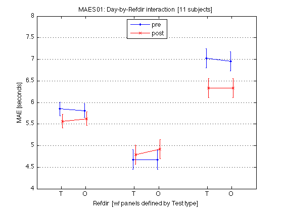
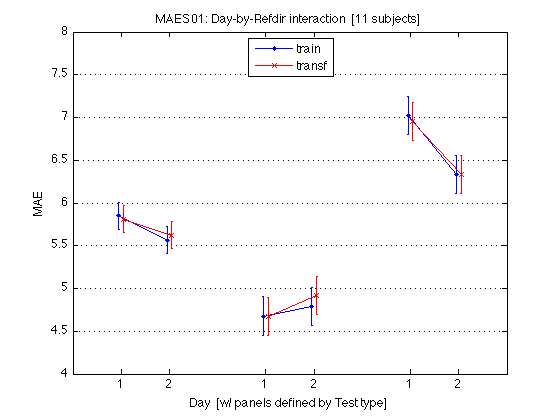
180: Plot the Day-by-Refdir interaction averaged across all MAES01 subjects
See figure-caption comment at the end of this section See Section 430 for the MAESpec02 analog.
x = [1 2] ;
AX = [0 9 4 8] ;           % for the group-level plots
ax = [0 9 2 11] ;          % for the individual plots
xtick = [1 2 4 5 7 8] ;
xticklabel_TO = 'T|O|T|O|T|O' ;
xticklabel_SD = 'S|D|S|D|S|D' ;
xticklabel_12 = '1|2|1|2|1|2' ;

M = mean(mean_MAE_by_sbj.MAES01_all_cells) / msec2sec ; % [1x8]
CI90 = mean_MAE_by_sbj.MAES01_grand_CI90 .* [1 1] ;

% The groups in each panel are defined by Test_type
DxR_static = M(V1.static) ;   % [1x4]
DxR_dynamic = M(V1.dynamic) ; % [1x4]
DxR = (DxR_static+DxR_dynamic)/2 ;

clf ; hold on ;
errorbar(x-.05,DxR(V1.pretest4T),CI90/sqrt(2),'b.-') ;
errorbar(x+.05,DxR(V1.posttest4T),CI90/sqrt(2),'rx-') ;

errorbar(x-.05+3,DxR_static(V1.pretest4T),CI90,'b.-') ;
errorbar(x+.05+3,DxR_static(V1.posttest4T),CI90,'rx-') ;

errorbar(x-.05+6,DxR_dynamic(V1.pretest4T),CI90,'b.-') ;
errorbar(x+.05+6,DxR_dynamic(V1.posttest4T),CI90,'rx-') ;
hold off ; box on ;
axis(AX) ;
set(gca,'xtick',xtick,'xticklabel',xticklabel_TO,'Ygrid','on') ;

title('MAES01: Day-by-Refdir interaction  [11 subjects]') ;
legend('pre','post','location','North') ;
xlabel('Refdir  [w/ panels defined by Test type]') ;
ylabel('MAE [seconds]') ;

clearvars M CI90 DxR_static DxR_dynamic DxR ;

% The leftmost group plots the DxR interaction (averaged across test_type).
% The middle group plots the DxR for STATIC tests.
% The rightmost group plots the DxR for DYNAMIC tests.
% Xticks: T=trained refdir, O=orthogonal refdir.
% Blue lines = PRETEST; Red lines = POSTTEST.
% Error bars are 90% CIs within subjects.
%
% All segments are nearly horizontal, which indicates that the main effect
% of refdir is weak. More importantly, the blue and red segments are nearly
% parallel, which indicates that practice ("Day") does not interact
% significantly with refdir.
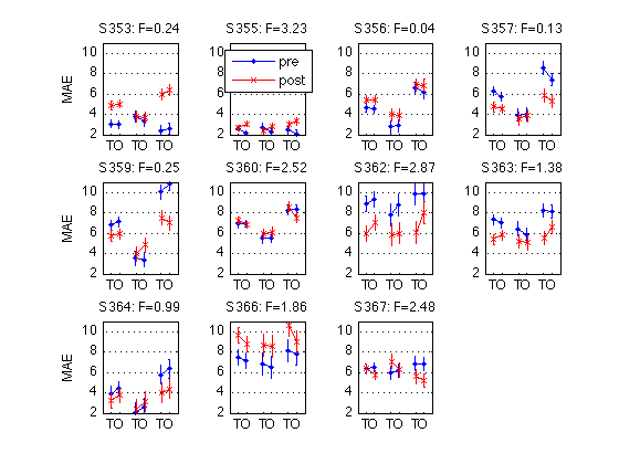
190: Plot the Day-by-Refdir interaction for each individual MAES01 subject
See figure-caption comment at the end of this section See Section 440 for the MAESpec02 analog.
for k = 1:N_MAES01_sbj
    M = D1(k).cell_nanmean_MAE / msec2sec ; % [1x8], see indices above
    CI90 = D1(k).indiv_ANOVA.CI90_cell_means .* [1 1] ;

    % The groups in each panel are defined by Test_type
    DxR_static = M(V1.static) ;   % [1x4]
    DxR_dynamic = M(V1.dynamic) ; % [1x4]
    DxR = (DxR_static+DxR_dynamic)/2 ;

    subplot(3,4,k) ;
    cla ; hold on ;
    errorbar(x-.05,DxR(V1.pretest4T),CI90/sqrt(2),'b.-') ;
    errorbar(x+.05,DxR(V1.posttest4T),CI90/sqrt(2),'rx-') ;

    errorbar(x-.05+3,DxR_static(V1.pretest4T),CI90,'b.-') ;
    errorbar(x+.05+3,DxR_static(V1.posttest4T),CI90,'rx-') ;

    errorbar(x-.05+6,DxR_dynamic(V1.pretest4T),CI90,'b.-') ;
    errorbar(x+.05+6,DxR_dynamic(V1.posttest4T),CI90,'rx-') ;
    hold off ; box on ;
    axis(ax) ;
    set(gca,'xtick',xtick,'xticklabel',xticklabel_TO,'Ygrid','on') ;

    title(sprintf('S%3d: F=%.2f',D1(k).sbj,MAES01_psy_F(k,V1.R_at_POST))) ;

    if (k==2) ; legend('pre','post','location','North') ; end
    if (mod(k,4)==1) ; ylabel('MAE') ; end
end
clearvars M CI90 DxR_static DxR_dynamic DxR ;

% The leftmost group in each panel plots the DxR interaction (averaged
% across test_type). Xticks: T=trained refdir, O=orthogonal refdir.
% The middle group plots the DxR for STATIC tests.
% The rightmost group plots the DxR for DYNAMIC tests.
% Blue lines = PRETEST; Red lines = POSTTEST.
% The title reports the F value for Refdir at POSTTEST for this subject.
%
% All segments are nearly horizontal, which indicates that the main effect
% of refdir is weak. More importantly, the blue and red segments are nearly
% parallel, which indicates that practice ("Day") does not interact
% significantly with refdir.
200: Plot the (grand) Day-by-Refdir interaction the other way around
See figure-caption comment at the end of this section. See Section 330 for publication-quality version containing the present figure as a subfigure. See Section 450 for the MAESpec02 analog.
M = mean(mean_MAE_by_sbj.MAES01_all_cells) / msec2sec ; % [1x8]
CI90 = repmat(mean_MAE_by_sbj.MAES01_grand_CI90,1,2)    % [1x2]

% The groups in each panel are still defined by Test_type
DxR_static = M(V1.static)          % [1x4]
DxR_dynamic = M(V1.dynamic)        % [1x4]
DxR = (DxR_static+DxR_dynamic)/2

clf ; hold on ;
errorbar(x-.05,DxR(V1.train4T),CI90/sqrt(2),'b.-') ;
errorbar(x+.05,DxR(V1.transf4T),CI90/sqrt(2),'rx-') ;

errorbar(x-.05+3,DxR_static(V1.train4T),CI90,'b.-') ;
errorbar(x+.05+3,DxR_static(V1.transf4T),CI90,'rx-') ;

errorbar(x-.05+6,DxR_dynamic(V1.train4T),CI90,'b.-') ;
errorbar(x+.05+6,DxR_dynamic(V1.transf4T),CI90,'rx-') ;
hold off ; box on ;
axis(AX) ;
set(gca,'xtick',xtick,'xticklabel',xticklabel_12,'Ygrid','on') ;

title('MAES01: Day-by-Refdir interaction  [11 subjects]') ;
legend('train','transf','location','North') ;
xlabel('Day  [w/ panels defined by Test type]') ;
ylabel('MAE') ;

clearvars M CI90 DxR_static DxR_dynamic DxR ;

% The leftmost group plots the DxR interaction (averaged across test_type).
% The middle group plots the DxR for STATIC tests.
% The rightmost group plots the DxR for DYNAMIC tests.
% Xticks: 1=pretest, 2=posttest
% Blue lines = TRAIN refdir; Red lines = TRANSF (=orthogonal) refdir.
% Error bars are 90% CIs within subjects.
%
% The blue and red segments are close to each other, which indicates that
% the main effect of refdir is weak. More importantly, the blue and red
% segments are nearly parallel, which indicates that practice ("Day")
% does not interact significantly with refdir.
CI90 =

    0.2233    0.2233


DxR_static =

    4.6776    4.6696    4.7939    4.9179


DxR_dynamic =

    7.0230    6.9517    6.3300    6.3292


DxR =

    5.8503    5.8107    5.5620    5.6236
210: Plot the individual Day-by-Refdir interactions the other way around
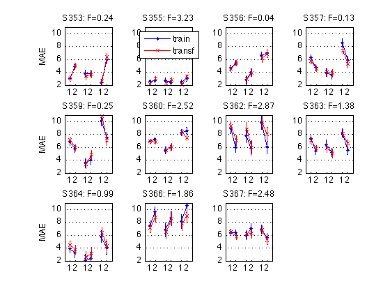
See figure-caption comment at the end of this section See Section 330 for a publication-quality version. See Section 460 for the MAESpec02 analog.
for k = 1:N_MAES01_sbj
    M = D1(k).cell_nanmean_MAE / msec2sec ; % [1x8], see indices above
    CI90 = D1(k).indiv_ANOVA.CI90_cell_means .* [1 1] ;

    % The groups in each panel are still defined by Test_type
    DxR_static = M(V1.static) ;   % [1x4]
    DxR_dynamic = M(V1.dynamic) ; % [1x4]
    DxR = (DxR_static+DxR_dynamic)/2 ;

    subplot(3,4,k) ;
    cla ; hold on ;
    errorbar(x-.05,DxR(V1.train4T),CI90/sqrt(2),'b.-') ;
    errorbar(x+.05,DxR(V1.transf4T)',CI90/sqrt(2),'rx-') ;

    errorbar(x-.05+3,DxR_static(V1.train4T)',CI90,'b.-') ;
    errorbar(x+.05+3,DxR_static(V1.transf4T)',CI90,'rx-') ;

    errorbar(x-.05+6,DxR_dynamic(V1.train4T)',CI90,'b.-') ;
    errorbar(x+.05+6,DxR_dynamic(V1.transf4T)',CI90,'rx-') ;
    hold off ; box on ;
    axis(ax) ;
    set(gca,'xtick',xtick,'xticklabel',xticklabel_12,'Ygrid','on') ;

    title(sprintf('S%3d: F=%.2f',D1(k).sbj,MAES01_psy_F(k,V1.R_at_POST))) ;

    if (k==2) ; legend('train','transf','location','North') ; end
    if (mod(k,4)==1) ; ylabel('MAE') ; end
end
clearvars M CI90 DxR_static DxR_dynamic DxR ;

% The leftmost group in each panel plots the DxR interaction (averaged
% across test_type). Xticks: 1=pretest, 2=posttest
% The middle group plots the DxR for STATIC tests.
% The rightmost group plots the DxR for DYNAMIC tests.
% Blue lines = TRAIN refdir; Red lines = TRANSF (=orthogonal) refdir.
% The title reports the F value for Refdir at POSTTEST for this subject.
%
% The blue and red segments are close to each other, which indicates that
% the main effect of refdir is weak. More importantly, the blue and red
% segments are nearly parallel, which indicates that practice ("Day")
% does not interact significantly with refdir.
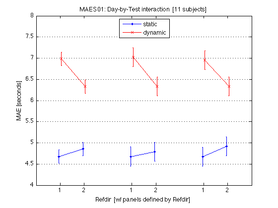
220: Plot the Day-by-Test interaction averaged across all MAES01 subjects
See figure caption in comment at the end of this section
M = mean(mean_MAE_by_sbj.MAES01_all_cells) / msec2sec ; % [1x8]
CI90 = mean_MAE_by_sbj.MAES01_grand_CI90 .* [1 1] ;

% The groups in each panel are defined by Refdir
DxT_train = M(V1.train) ;   % [1x4]
DxT_transf = M(V1.transf) ; % [1x4]
DxT = (DxT_train+DxT_transf)/2 ;

clf ; hold on ;
errorbar(x-.05,DxT(V1.static4R),CI90/sqrt(2),'b.-') ;
errorbar(x+.05,DxT(V1.dynamic4R),CI90/sqrt(2),'rx-') ;

errorbar(x-.05+3,DxT_train(V1.static4R),CI90,'b.-') ;
errorbar(x+.05+3,DxT_train(V1.dynamic4R),CI90,'rx-') ;

errorbar(x-.05+6,DxT_transf(V1.static4R),CI90,'b.-') ;
errorbar(x+.05+6,DxT_transf(V1.dynamic4R),CI90,'rx-') ;
hold off ; box on ;
axis(AX) ;
set(gca,'xtick',xtick,'xticklabel',xticklabel_12,'Ygrid','on') ;

title('MAES01: Day-by-Test interaction  [11 subjects]') ;
legend('static','dynamic','location','North') ;
xlabel('Refdir  [w/ panels defined by Refdir]') ;
ylabel('MAE [seconds]') ;

clearvars M CI90 DxT_train DxT_transf DxT ;

% The leftmost group plots the DxT interaction (averaged across refdirs).
% The middle group plots the DxT for TRAIN refdir.
% The rightmost group plots the DxT for TRANSF (=orthogonal) refdir.
% Xticks: 1=pretest, 2=posttest
% Blue lines = STATIC; Red lines = DYNAMIC.
% Error bars are 90% CIs within subjects.
%
% The red segments are far above the blue segments, indicating the mean
% effect of the Test_type factor -- dynamic tests produce longer MAEs.
% This difference diminishes somewhat (but remains strong) at posttest.
% The three panels are the same --> Refdir does not make much difference.
230: Plot the Day-by-Test interaction for each individual MAES01 subject
See figure caption in comment at the end of this section
for k = 1:N_MAES01_sbj
    M = D1(k).cell_nanmean_MAE / msec2sec ; % [1x8], see indices above
    CI90 = D1(k).indiv_ANOVA.CI90_cell_means .* [1 1] ;

    % The groups in each panel are defined by Refdir
    DxT_train = M(V1.train) ;   % [1x4]
    DxT_transf = M(V1.transf) ; % [1x4]
    DxT = (DxT_train+DxT_transf)/2 ;

    subplot(3,4,k) ;
    cla ; hold on ;
    errorbar(x-.05,DxT(V1.static4R),CI90/sqrt(2),'b.-') ;
    errorbar(x+.05,DxT(V1.dynamic4R),CI90/sqrt(2),'rx-') ;

    errorbar(x-.05+3,DxT_train(V1.static4R),CI90,'b.-') ;
    errorbar(x+.05+3,DxT_train(V1.dynamic4R),CI90,'rx-') ;

    errorbar(x-.05+6,DxT_transf(V1.static4R),CI90,'b.-') ;
    errorbar(x+.05+6,DxT_transf(V1.dynamic4R),CI90,'rx-') ;
    hold off ; box on ;
    axis(ax) ;
    set(gca,'xtick',xtick,'xticklabel',xticklabel_12,'Ygrid','on') ;

    title(sprintf('S%3d: F=%.2f',D1(k).sbj,MAES01_ind_F(k,5))) ;

    if (k==2) ; legend('stat','dyn','location','North') ; end
    if (mod(k,4)==1) ; ylabel('MAE') ; end
end
clearvars M CI90 DxT_train DxT_transf DxT ;

% The leftmost group in each panel plots the DxT interaction (averaged
% across refdirs). Xticks: 1=pretest, 2=posttest
% The middle group plots the DxT for TRAIN refdir.
% The rightmost group plots the DxT for TRANSF (=orthogonal) refdir.
% Blue lines = PRETEST; Red lines = POSTTEST.
% The title reports the F value for the DxT interaction for this subject.
%
% The red segments tend to be above the blue segments, indicating the mean
% effect of the Test_type factor -- dynamic tests produce longer MAEs.
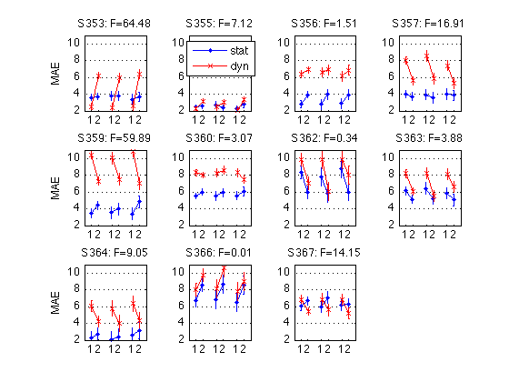
240: Plot the grand Day-by-Test interaction the other way around
See figure caption in comment at the end of this section
M = mean(mean_MAE_by_sbj.MAES01_all_cells) / msec2sec ; % [1x8]
CI90 = mean_MAE_by_sbj.MAES01_grand_CI90 .* [1 1] ;

% The groups in each panel are still defined by Refdir
DxT_train = M(V1.train) ;   % [1x4]
DxT_transf = M(V1.transf) ; % [1x4]
DxT = (DxT_train+DxT_transf)/2 ;

clf ; hold on ;
errorbar(x-.05,DxT(V1.pretest4R),CI90/sqrt(2),'b.-') ;
errorbar(x+.05,DxT(V1.posttest4R),CI90/sqrt(2),'rx-') ;

errorbar(x-.05+3,DxT_train(V1.pretest4R),CI90,'b.-') ;
errorbar(x+.05+3,DxT_train(V1.posttest4R),CI90,'rx-') ;

errorbar(x-.05+6,DxT_transf(V1.pretest4R),CI90,'b.-') ;
errorbar(x+.05+6,DxT_transf(V1.posttest4R),CI90,'rx-') ;
hold off ; box on ;
axis(AX) ;
set(gca,'xtick',xtick,'xticklabel',xticklabel_SD,'Ygrid','on') ;

title('MAES01: Day-by-Test interaction  [11 subjects]') ;
legend('pretest','posttest','location','North') ;
xlabel('Refdir  [w/ panels defined by Refdir]') ;
ylabel('MAE [seconds]') ;

clearvars M CI90 DxT_train DxT_transf DxT ;

% The leftmost group plots the DxT interaction (averaged across refdirs).
% The middle group plots the DxT for TRAIN refdir.
% The rightmost group plots the DxT for TRANSF (=orthogonal) refdir.
% Xticks: S=static, D=dynamic test.
% Blue lines = PRETEST; Red lines = POSTTEST.
% Error bars are 90% CIs within subjects.
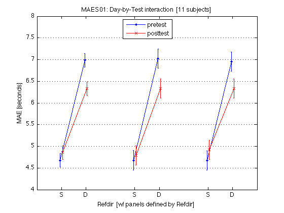
250: Plot the individual Day-by-Test interaction the other way around
See figure-caption comment at the end of this section
for k = 1:N_MAES01_sbj
    M = D1(k).cell_nanmean_MAE / msec2sec ; % [1x8], see indices above
    CI90 = D1(k).indiv_ANOVA.CI90_cell_means .* [1 1] ;

    % The groups in each panel are still defined by Refdir
    DxT_train = M(V1.train) ;   % [1x4]
    DxT_transf = M(V1.transf) ; % [1x4]
    DxT = (DxT_train+DxT_transf)/2 ;

    subplot(3,4,k) ;
    cla ; hold on ;
    errorbar(x-.05,DxT(V1.pretest4R),CI90/sqrt(2),'b.-') ;
    errorbar(x+.05,DxT(V1.posttest4R),CI90/sqrt(2),'rx-') ;

    errorbar(x-.05+3,DxT_train(V1.pretest4R),CI90,'b.-') ;
    errorbar(x+.05+3,DxT_train(V1.posttest4R),CI90,'rx-') ;

    errorbar(x-.05+6,DxT_transf(V1.pretest4R),CI90,'b.-') ;
    errorbar(x+.05+6,DxT_transf(V1.posttest4R),CI90,'rx-') ;
    hold off ; box on ;
    axis(ax) ;
    set(gca,'xtick',xtick,'xticklabel',xticklabel_SD,'Ygrid','on') ;

    title(sprintf('S%3d: F=%.2f',D1(k).sbj,MAES01_ind_F(k,5))) ;

    if (k==2) ; legend('pre','post','location','North') ; end
    if (mod(k,4)==1) ; ylabel('MAE') ; end
end
clearvars M CI90 DxT_train DxT_transf DxT ;

% The leftmost group in each panel plots the DxT interaction (averaged
% across refdirs). Xticks: S=static, D=dynamic test.
% The middle group plots the DxT for TRAIN refdir.
% The rightmost group plots the DxT for TRANSF (=orthogonal) refdir.
% Blue lines = PRETEST; Red lines = POSTTEST.
% The title reports the F value for the DxT interaction for this subject.
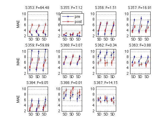
260: Within-subject, grand ANOVA for MAESpec01
All missing values have been filled in. This affects only the df's for the last two rows ('err' and 'Totl'), however. The rest of the analysis could just as well have been done on the cell means instead on the raw MAE durations. Thus, the only benefit of having 21 replications per cell is to reduce the measurement error of the corresponding MAE. The variance of these measurements does not inform the F ratios for the effects of interest (because each of them uses the corresponding factor-by-subject interaction for the error term). Unfortunately, this means that all tests are done with only 10 degrees of freedom (N_sbj-1).
See Section 600 for the MAESpec02 analog.
data = cat(1,D1.new_data) ;  % [1848x10]; 1848=N_MAES01_sbj*N_trials
sbj = repmat(1:N_MAES01_sbj,MAE_design.N_trials,1) ;  % [168x11]

DV = data(:,J.MAE) / msec2sec ;   % [1848x1] missing values filled in
IVs = [data(:,[J.day J.refdir J.test_type]) , sbj(:)] ; % [1848x4]
names = 'DRTS' ;

%- Partition the variance and print the ANOVA table
st = anova(DV,IVs,names,1) ;

%- Calculate Fs for the factors of interest
num = [1 2  3,  5  6  8, 11] ;   % [D  R  T , DR  DT  RT , DRT ]
den = [7 9 10, 12 13 14, 15] ;   % [DS RS TS, DRS DTS RTS, DRTS]
st.numerator = num ;
st.denominator = den ;
assert(all(st.df(num)==1)) ;
assert(all(st.df(den)==N_MAES01_sbj-1)) ;  % That's why power is low :(

st.effects = st.labels(num) ;
st.error_terms = st.labels(den) ;
st.errof_dfs = st.df(den) ;

st.MS_numerator = st.MS(num) ;
st.MS_err = st.MS(den) ;
st.morm_MS_err = st.MS_err ./ mean(DV)^2 ; % mean(DV)=5.7067; M^2=32.5668

st.F = st.MS(num) ./ st.MS(den) ;
st.t = sqrt(st.F) ;
st.p = 1-fcdf(st.F,st.df(num),st.df(den)) ;
Partitioning the sum of squares...

 k Source         SumSq   eta2[%]     df        MeanSq
------------------------------------------------------
 1    D          29.127     0.18       1       29.1269
 2    R           0.124     0.00       1        0.1241
 3    T        1635.248    10.19       1     1635.2480
 4    S        5087.130    31.69      10      508.7130
 5   DR           1.170     0.01       1        1.1698
 6   DT          87.798     0.55       1       87.7983
 7   DS         878.205     5.47      10       87.8205
 8   RT           0.900     0.01       1        0.8998
 9   RS          65.513     0.41      10        6.5513
10   TS         898.825     5.60      10       89.8825
11  DRT           0.153     0.00       1        0.1534
12  DRS          29.378     0.18      10        2.9378
13  DTS         437.219     2.72      10       43.7219
14  RTS          33.708     0.21      10        3.3708
15 DRTS          49.311     0.31      10        4.9311
16  err        6817.904    42.47    1760        3.8738
17 Totl       16051.714   100.00    1847        8.6907
------------------------------------------------------
270: Effect sizes for the grand ANOVA
Done according to Sections 16.3, 18.5, and 21.4 in Keppel & Wickens (2004). They write that "the situation is complicated" (p. 426). "When the design contains 2 within-sbj factors [and we have 3], ... we can only determine a range for the effect size (Dodd & Schultz, 1973)."
Here, we'll calculate both the lower and the upper bounds in Eq.18.9. They differ only in the number of observations in the denominator. I've tried to generalize from two-way to three-way formulas (by treating two-factor combinations as a single factor with more levels), but there are no guarantees I got it exactly right. These things are tricky!
N_lower = st.df(end)+1 ;  % abcn=168: lower-bound in Eq.18.9, same for all factors
N_upper = N_reps_per_cell .* (st.df(num)+1) ; % an=42: upper-bound in Eq.18.9

%- Calculate partial omega-squared
w2 = st.df(num) .* (st.F-1) ;
w2 = max(0,w2) ;  % F values < 1.0 are entirely due to sampling error.

st.partial_omega2_lower = w2./(w2+N_lower) ;  % Eq. 18.9, left panel
st.partial_omega2_upper = w2./(w2+N_upper) ;  % Eq. 18.9, right panel

%- Calculate complete omega-squared
st.complete_omega2_lower = w2./(sum(w2)+N_lower) ;  % Eq. 21.9
st.complete_omega2_upper = w2./(sum(w2)+N_upper) ;  % Eq. 21.9

%- Store and move on
MAES01_grand_ANOVA = st

clearvars st DV IVs names num den ;

% Conclusion:  The only significant effect is that of the Test_type factor.
% The dynamic MAE last ~2 seconds longer than the static MAE, on average
% (~6.8 vs. ~4.8 seconds, respectively). See the DxT figures above.
%
% The Refdir factor is not significant (F=0.0189, t=0.1376, p=.893).
% The DxR interaction is not signif. either (F=0.3982, t=0.6310, p=.542).
% Because both F values are < 1, the effect-size estimates are 0. Duh!
% "The study gives no reliable info about the true means at all." (K&W,p.171)
MAES01_grand_ANOVA =

                      lbl: [17x4 char]
                   labels: {1x17 cell}
                       SS: [1x17 double]
                       df: [1 1 1 10 1 1 10 1 10 10 1 10 10 10 10 1760 1847]
                       MS: [1x17 double]
                numerator: [1 2 3 5 6 8 11]
              denominator: [7 9 10 12 13 14 15]
                  effects: {'   D'  '   R'  '   T'  '  DR'  '  DT'  '  RT'  ' DRT'}
              error_terms: {'  DS'  '  RS'  '  TS'  ' DRS'  ' DTS'  ' RTS'  'DRTS'}
                errof_dfs: [10 10 10 10 10 10 10]
             MS_numerator: [29.1269 0.1241 1.6352e+03 1.1698 87.7983 0.8998 0.1534]
                   MS_err: [87.8205 6.5513 89.8825 2.9378 43.7219 3.3708 4.9311]
              morm_MS_err: [2.6966 0.2012 2.7599 0.0902 1.3425 0.1035 0.1514]
                        F: [0.3317 0.0189 18.1932 0.3982 2.0081 0.2669 0.0311]
                        t: [0.5759 0.1376 4.2653 0.6310 1.4171 0.5167 0.1764]
                        p: [0.5774 0.8933 0.0016 0.5422 0.1869 0.6166 0.8635]
     partial_omega2_lower: [0 0 0.0092 0 5.4522e-04 0 0]
     partial_omega2_upper: [0 0 0.2905 0 0.0234 0 0]
    complete_omega2_lower: [0 0 0.0092 0 5.4019e-04 0 0]
    complete_omega2_upper: [0 0 0.2856 0 0.0167 0 0]
280: Don't do contrast-based grand ANOVA for MAESpec01
Inspired by Section 155 above, one might be tempted to repartition the SS for (Refdir + DxR) into (R_at_PRE + R_at_POST). However, the DxR interaction so completely dominates the Refdir main effect in these data that shifting the variance around can only decrease the F ratios. As DxR is not significant (F=0.3982), the contrasts cannot be significant either.
For future reference: (Keppel & Wickens, 2004, p.412) "When we have a [simple] effect involving a portion of within-subject data, we isolate those data and analyze them separately.
290: Power analysis for the grand ANOVA for MAESpec01
Build on the individual power analysis from Section 165. Two things change: MS_err and df_err. And, of course, we don't have the luxury of 11 independent replications.
The contrasts for Refdir at PRE and POST do not apply. Luckily, their indice come last, and so dropping them won't mess up the bookkeeping. (Actually, we could have dropped V1.Day too, but that would mess it up.)
%- Copy the contrasts from the individual power analysis from Section 165
idx = [V1.Day V1.Refdir V1.DxR] ;   %
pwr1g.contrast_names = pwr1.contrast_names(idx) ;
pwr1g.contrasts = pwr1.contrasts(:,idx) ;

pwr1g.hyp_change = pwr1.hyp_change ;          % [1x6]
pwr1g.hyp_MAE_means = pwr1.hyp_MAE_means ;    % [6x8]
pwr1g.hyp_psy = pwr1.hyp_psy(:,idx) ;         % [6x3]
pwr1g.hyp_s2_psy = pwr1.hyp_s2_psy(idx,:) ;   % [3x6]

%- The MS_err now is the corresponding interaction with subjects
% For comparison pwr1.median_norm_MS_err==0.0992. This is comparable to
% what we have here for DxR.  However, MS_err for the Refdir factor here
% is two times worse.  (I'm not quite sure what's going on with Day.)
norm_MS_err_within = NaN(1,length(idx)) ;
norm_MS_err_within(V1.Day) = MAES01_grand_ANOVA.morm_MS_err(1) ;
norm_MS_err_within(V1.Refdir) = MAES01_grand_ANOVA.morm_MS_err(2) ;
norm_MS_err_within(V1.DxR) = MAES01_grand_ANOVA.morm_MS_err(4) ;
pwr1g.norm_MS_err_within = norm_MS_err_within   % [1x3]


% TO DO...  @@@ @@@
clearvars idx :   % @@@@
pwr1g =

        contrast_names: {'Day'  'Refdir'  'DxR'}
             contrasts: [8x3 double]
            hyp_change: [0.0500 0.1000 0.1500 0.2000 0.2500 0.3000]
         hyp_MAE_means: [6x8 double]
               hyp_psy: [6x3 double]
            hyp_s2_psy: [3x6 double]
    norm_MS_err_within: [2.6966 0.2012 0.0902]
300: Within-subject, grander ANOVA for MAESpec01
Add the 'position' factor -- it has 21 levels and counts the number of times a particular stimulus has been tested so far. The 4 sequences for the 2 different directions x 2 test_types are interleaved at random, but this is ignored in this analysis. Still, the position can serve as a rough time variable, suitable for learning curves, etc. Thus, it is interesting to see whether it has a significant main effect and whether in interacts with the other factors.
The MS_within for the other factors are not changed. So, the above ANOVA results still apply in full. We're only testing P here.
DV = data(:,J.MAE) / msec2sec ;   % [1848x1] missing values filled in
IVs = [data(:,[J.day J.refdir J.test_type J.position]) , sbj(:)] ; % [1848x5]
names = 'DRTPS' ;

%- Partition the variance and print the ANOVA table
%  Note that all the fields not involving P are the same as before.
st = anova(DV,IVs,names,1)

%- Calculate Fs for the factors of interest
num = [ 4,  8 11 13, 17 19 22, 26] ;   % [P , DP  RP  TP , DRP  DTP  RTP , DRTP ]
den = [15, 21 24 25, 28 29 30, 31] ;   % [PS, DPS RPS TPS, DRPS DTPS RTPS, DRTPS]
st.numerator = num ;
st.denominator = den ;
assert(all(st.df(num)==(N_reps_per_cell-1))) ;
assert(all(st.df(den)==((N_reps_per_cell-1)*(N_MAES01_sbj-1)))) ;  % HIGH power
st.effects = st.labels(num) ;
st.error_terms = st.labels(den) ;

st.MS_numerator = st.MS(num) ;
st.MS_err = st.MS(den) ;
st.MS_err_relative  = st.MS_err ./ mean(DV).^2 ;

st.F = st.MS(num) ./ st.MS(den) ;
st.p = 1-fcdf(st.F,st.df(num),st.df(den)) ;

MAES01_grandest_ANOVA = st
clearvars st DV IVs names num den ;

% Conclusion: The only significant effect involving Period is its
% interaction with Day (F=3.3103, p<.000008).  Note that the terms
% involving the RxP conjuction still aren't significant.  DxRxP in
% particular, has F=1.0009, p=.1377.  It would be interesting to do a
% power analysis for this given that there are 200 error df's.
Partitioning the sum of squares...

 k Source         SumSq   eta2[%]     df        MeanSq
------------------------------------------------------
 1     D          29.127     0.18       1       29.1269
 2     R           0.124     0.00       1        0.1241
 3     T        1635.248    10.19       1     1635.2480
 4     P         138.867     0.87      20        6.9433
 5     S        5087.130    31.69      10      508.7130
 6    DR           1.170     0.01       1        1.1698
 7    DT          87.798     0.55       1       87.7983
 8    DP         353.000     2.20      20       17.6500
 9    DS         878.205     5.47      10       87.8205
10    RT           0.900     0.01       1        0.8998
11    RP          58.984     0.37      20        2.9492
12    RS          65.513     0.41      10        6.5513
13    TP         112.697     0.70      20        5.6349
14    TS         898.825     5.60      10       89.8825
15    PS        1047.120     6.52     200        5.2356
16   DRT           0.153     0.00       1        0.1534
17   DRP          55.835     0.35      20        2.7918
18   DRS          29.378     0.18      10        2.9378
19   DTP          41.928     0.26      20        2.0964
20   DTS         437.219     2.72      10       43.7219
21   DPS        1066.355     6.64     200        5.3318
22   RTP          58.932     0.37      20        2.9466
23   RTS          33.708     0.21      10        3.3708
24   RPS         522.810     3.26     200        2.6141
25   TPS         819.311     5.10     200        4.0966
26  DRTP          66.102     0.41      20        3.3051
27  DRTS          49.311     0.31      10        4.9311
28  DRPS         557.878     3.48     200        2.7894
29  DTPS         887.336     5.53     200        4.4367
30  RTPS         524.896     3.27     200        2.6245
31 DRTPS         505.853     3.15     200        2.5293
32 Error          -0.000    -0.00       0        0.0000
33 Total       16051.714   100.00    1847        8.6907
------------------------------------------------------

st =

       lbl: [33x5 char]
    labels: {1x33 cell}
        SS: [1x33 double]
        df: [1 1 1 20 10 1 1 20 10 1 20 10 20 10 200 1 20 10 20 10 200 20 10 200 200 20 10 200 200 200 200 0 1847]
        MS: [1x33 double]


MAES01_grandest_ANOVA =

                lbl: [33x5 char]
             labels: {1x33 cell}
                 SS: [1x33 double]
                 df: [1x33 double]
                 MS: [1x33 double]
          numerator: [4 8 11 13 17 19 22 26]
        denominator: [15 21 24 25 28 29 30 31]
            effects: {'    P'  '   DP'  '   RP'  '   TP'  '  DRP'  '  DTP'  '  RTP'  ' DRTP'}
        error_terms: {'   PS'  '  DPS'  '  RPS'  '  TPS'  ' DRPS'  ' DTPS'  ' RTPS'  'DRTPS'}
       MS_numerator: [6.9433 17.6500 2.9492 5.6349 2.7918 2.0964 2.9466 3.3051]
             MS_err: [5.2356 5.3318 2.6141 4.0966 2.7894 4.4367 2.6245 2.5293]
    MS_err_relative: [0.1608 0.1637 0.0803 0.1258 0.0857 0.1362 0.0806 0.0777]
                  F: [1.3262 3.3103 1.1282 1.3755 1.0009 0.4725 1.1227 1.3068]
                  p: [0.1656 7.9782e-06 0.3232 0.1377 0.4628 0.9742 0.3286 0.1778]
310: Plot the Day-by-Period interaction averaged across all MAES01 subjects
See figure caption in comment at the end of this section
[s,k] = split(data(:,J.MAE_duration)/msec2sec,data(:,[J.day J.position])) ;
d = [k aggreg(s,'nanmean')]  ;   % [42x3]: [day period mnMAE]

d1=(d(:,1)==enum.PRETEST) ;
d2=(d(:,1)==enum.POSTTEST) ;

clf
plot(d(d1,2),d(d1,3),'b.-',d(d2,2),d(d2,3),'rx-') ;
axis([0 N_reps_per_cell+1 4 8]) ; grid on ;
xlabel('Position') ; ylabel('MAE [seconds]') ;
title('MAES01: Day-by-Position interaction  [11 subjects]') ;
legend('Pretest','Posttest','location','NorthEast') ;

clearvars s k d d1 d2 ;
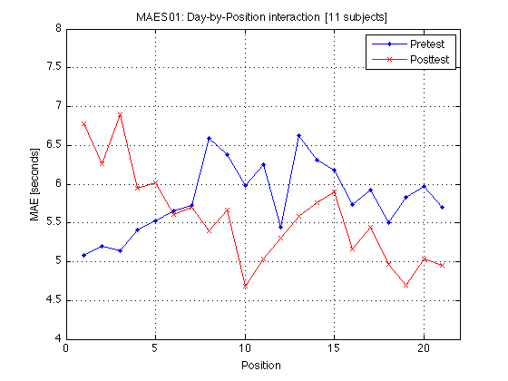
330: Make a publication-quality figure of the MAE results, MAESpec01
Combines the figures from Sections 200 and 210 above into a single figure intended for publication. Exported to .eps format, with antialiasing, etc. AAP, 2011-03-12
STATIC and DYNAMIC data are shown side by side on each plot, but the average (STATIC+DYNAMIC)/2 is not shown, unlike in Sect 200 and 210.
See Section 650 below for the MAESpec02 analog.
xtick = [1 2 4 5] ;
xticklabel_12 = 'pre|post|pre|post' ;
MarkerSize = 8 ;
LineWidth = 1.2 ;

%-- Open a (big) figure window in preparation to call export_fig below
clf ;
set(gcf,'Color','none') ;   % set transparent background for figure
set(gcf,'Position',[1 1 1000 600]) ;


%-- Group-level plot, twice as big as the individual plots
% This is a refinement of the plot in Section 200 above.

M = mean(mean_MAE_by_sbj.MAES01_all_cells) / msec2sec ;  % [1x8]
CI90 = repmat(mean_MAE_by_sbj.MAES01_grand_CI90,1,2) ;   % [1x2]

% The groups in each panel are still defined by Test_type
DxR_static = M(V1.static)   ;       % [1x4]
DxR_dynamic = M(V1.dynamic) ;       % [1x4]

subplot(2,2,1) ;   % big plot  @@@ needs manual adjustment

hold on ;
h = errorbar(x-.05,DxR_static(V1.train4T),CI90,'ro-') ;
set(h,'MarkerSize',MarkerSize,'LineWidth',LineWidth) ;
h = errorbar(x+.05,DxR_static(V1.transf4T),CI90,'bx--') ;
set(h,'MarkerSize',MarkerSize,'LineWidth',LineWidth) ;

h = errorbar(x-.05+3,DxR_dynamic(V1.train4T),CI90,'ro-') ;
set(h,'MarkerSize',MarkerSize,'LineWidth',LineWidth) ;
h = errorbar(x+.05+3,DxR_dynamic(V1.transf4T),CI90,'bx--') ;
set(h,'MarkerSize',MarkerSize,'LineWidth',LineWidth) ;
hold off ;

box on ;
axis([0 6 4 8]) ;
set(gca,'xtick',xtick,'xticklabel',xticklabel_12,'ytick',4:8) ; %,'Ygrid','on') ;

text(1.2,5.8,'Static') ; text(4,5.8,'Dynamic') ;
legend('Trained direction','Control  direction','location','NorthWest') ;
ylabel('MAE duration (seconds)') ;
%xlabel('Session') ;


%-- Individual plots, half the size of the group plot
% This is a refinement of the plot in Section 210 above.

% The group subplot above occupies cells 1,2,5, and 6 of this finer grid.
% The individual plots will be plotted at the following indices:
subplot_idx = [3 4, 7 8, 9:12, 13:15] ;    % cell #16 is empty

% Sort the subjects in increasing psy_F for the R_at_POST contrast:
F = MAES01_psy_F(:,V1.R_at_POST) ;
[~,sort_idx] = sort(F) ;

fprintf('Subplot idx = %s \n',mat2str(subplot_idx)) ;
fprintf('Sort idx = %s \n',mat2str(sort_idx')) ;
fprintf('Subject  = %s \n',mat2str([D1(sort_idx).sbj])) ;

for k = 1:N_MAES01_sbj
    sk = sort_idx(k) ;
    M = D1(sk).cell_nanmean_MAE / msec2sec ; % [1x8], see indices above
    CI90 = D1(sk).indiv_ANOVA.CI90_cell_means .* [1 1] ;

    % The groups in each panel are still defined by Test_type
    DxR_static = M(V1.static) ;   % [1x4]
    DxR_dynamic = M(V1.dynamic) ; % [1x4]

    subplot(4,4,subplot_idx(k)) ;
    cla ;

    hold on ;
    errorbar(x-.05,DxR_static(V1.train4T)',CI90,'ro-') ;
    errorbar(x+.05,DxR_static(V1.transf4T)',CI90,'bx--') ;

    errorbar(x-.05+3,DxR_dynamic(V1.train4T)',CI90,'ro-') ;
    errorbar(x+.05+3,DxR_dynamic(V1.transf4T)',CI90,'bx--') ;
    hold off ; box on ;

    % The individual diffs in overall MAE are so great that a vertical
    % adjustment is necessary
    if (k~=4)
        vert_adjust = [0 0 1 1].*max(4,round(mean(M))) ;
        axis([0 6 -4 4]+vert_adjust) ;
    else  % k==4 --> sk==5 --> sbj==359, who has anomalously big range
        axis([0 6 3 11]) ;
    end
    set(gca,'xtick',xtick,'xticklabel',[],'ytick',0:2:12) ; %,'Ygrid','on') ;

    %- To plot everybody on a fixed axis, use this instead:
    %axis([0 6 2 11]) ;
    %set(gca,'xtick',xtick,'xticklabel',[]) ; %,'Ygrid','on') ;

    title(sprintf('F=%.2f',F(sk))) ;

    %if (mod(subplot_idx(k),4)==1) ; ylabel('MAE') ; end
end

clearvars h k sk M CI90 DxR_static DxR_dynamic DxR F ;


%%%% To re-size the bigger panel, make Section 331 a separate section,
%%%% then execute Section 330 manually, resize manually, then execute
%%%% Section 331 manually.  AAP 2011-03-12
%%%% As it stands right now, the group panel won't be exactly aligned with
%%%% the smaller panels, but everything else is just like in the published
%%%% version.
%%%%
331: Write the figure to file, in PDF format, at high resolution
export_fig Exp1_DxR_fig.pdf -r150 -m3 -q100

close all ;
Subplot idx = [3 4 7 8 9 10 11 12 13 14 15]
Sort idx = [3 4 1 5 9 8 10 11 6 7 2]
Subject  = [356 357 353 359 364 363 366 367 360 362 355]
390: Done with all MAESpec01 analyses
clearvars data sbj x ax AX xtick xticklabel_12 xticklabel_SD xticklabel_TO ;

% As of 2010-07-22, completed up to this point
%
% ****************************************************************
% ****************************************************************
% ******  Most analyses above dealt with the data from the first
% ******  experiment (MAESpec01).  All analyses below this point
% ******  will deal with the data from the second expmt, MAESpec02.
% ****************************************************************
% ****************************************************************
% ****************************************************************
400: Individual ANOVAs for each MAES02 subject
Do an ANOVA for each individual subject. The error term is estimated from the 21 repetitions in each cell. There are 2 factors:
* day -- PRETEST vs POSTTEST -- denoted 'D' below
* refdir -- TRAIN, TRANSF, TRAIN180, TRANSF180 -- denoted 'R' below
In this design, the representation-modification hypothesis of perceptual learning predicts a significant DxR interaction.
% To illustrate, here's the ANOVA table for sbj 354:
%      k Source         SumSq   eta2[%]     df        MeanSq
%     ------------------------------------------------------
%      1    D           0.055     0.02       1        0.0549
%      2    R         165.845    46.86       3       55.2817
%      3   DR           4.714     1.33       3        1.5713
%      4  err         183.331    51.80     160        1.1458
%      5 Totl         353.944   100.00     167        2.1194
%     ------------------------------------------------------
%
% The df's of the error term should be decreased by 1 because there was
% 1 missing value.  The error MS and df are at index=8.  As all F's have
% only 1 df, they can be converted to t-statistics.  Can Rouder's Bayesian
% t-test be used to assert the nonsignificance of the DxR interaction?

DV = J.MAE ;  % divided by 1000 for convenience [msec-->sec]
IVs = [J.day, J.refdir] ;
names = 'DR' ;
tests_of_interest = 1:3 ;
err_idx = 4 ;

MAES02_ind_F = NaN(N_MAES02_sbj,length(tests_of_interest)) ;
MAES02_ind_p = NaN(N_MAES02_sbj,length(tests_of_interest)) ;
MAES02_ind_w2p = NaN(N_MAES01_sbj,length(tests_of_interest)) ;
MAES02_ind_w2c = NaN(N_MAES01_sbj,length(tests_of_interest)) ;

for k = 1:N_MAES02_sbj
    %- Retrieve data, missing values have been filled in
    nd = D2(k).new_data ;   % [168x10]
    N_missing = length(D2(k).NaN_idx) ;

    %- Partition the variance
    st = anova(nd(:,DV)/msec2sec,nd(:,IVs),names,0) ;

    %- Error term, pooled across all 8 cells
    assert(all(st.labels{err_idx}==' err')) ;   % sanity check
    MS_err = st.MS(err_idx) ;
    st.MS_err = MS_err ;                        % in seconds^2
    std_err = sqrt(MS_err/N_reps_per_cell) ;
    st.std_err_cell_means = std_err ;        % in seconds
    st.CI90_cell_means = std_err * tinv(.95,N_reps_per_cell-1) ; % two-tailed
    adj_df_err = st.df(err_idx) - N_missing ;
    st.adjusted_df_err = adj_df_err ;

    %- Calculate F
    st.F = st.MS(tests_of_interest) ./ MS_err ;
    MAES02_ind_F(k,:) = st.F ;

    st.p = 1-fcdf(st.F,st.df(tests_of_interest),adj_df_err) ;
    MAES02_ind_p(k,:) = st.p ;

    %- Calculate partial and complete omega-squared (Eqs. 21.7 & 21.8 in
    %  KeppelWickens04). The partial w^2 estimates the *population* ratio
    %  sigma^2_effect / (sigma^2_effect + sigma^2_error)   (Eq.21.6),
    %  where sigma^2_error is the error variance for the particular effect.
    %  The complete w^2 divides by the total variance of all effects.
    N = st.df(end)+1 ;  % 168 = total # of scores
    w2 = st.df(tests_of_interest).*(st.F(tests_of_interest)-1) ;
    w2 = max(0,w2) ;  % F values < 1.0 are entirely due to sampling error.
    st.partial_omega2 = w2./(w2+N) ;        % Eq. 21.7
    st.complete_omega2 = w2./(sum(w2)+N) ;  % Eq. 21.9
    MAES02_ind_w2p(k,:) = st.partial_omega2 ;
    MAES02_ind_w2c(k,:) = st.complete_omega2 ;

    %- Store and move on
    D2(k).indiv_ANOVA = st ;
end

clearvars k nd st MS_err std_err adj_df_err ;

%- Print a representative individual ANOVA.
%  This subject (#354) had no missing value and therefore
%  the adjusted_df_err is equal to df(err_idx)
fprintf('Representative individual ANOVA for sbj #%d\n',D2(1).sbj) ;
D2(1).indiv_ANOVA

% The critical value for df_num=3, df_err=160, p<.05, is:
fprintf('F(.95,3,160) = %.3f \n',finv(.95,3,160))
Representative individual ANOVA for sbj #354

ans =

                   lbl: [5x4 char]
                labels: {'   D'  '   R'  '  DR'  ' err'  'Totl'}
                    SS: [0.0549 165.8450 4.7138 183.3306 353.9443]
                    df: [1 3 3 160 167]
                    MS: [0.0549 55.2817 1.5713 1.1458 2.1194]
                MS_err: 1.1458
    std_err_cell_means: 0.2336
       CI90_cell_means: 0.4029
       adjusted_df_err: 160
                     F: [0.0479 48.2465 1.3713]
                     p: [0.8271 0 0.2535]
        partial_omega2: [0 0.4576 0.0066]
       complete_omega2: [0 0.4560 0.0036]

F(.95,3,160) = 2.661
402: Report MAES02 indiv_ANOVA results
labels = D2(1).indiv_ANOVA.labels(tests_of_interest) ;

[{'sbj'}   labels       labels]
[[D2.sbj]' MAES02_ind_F MAES02_ind_p]

fprintf('Distribution of Fs across the %d MAES02 subjects:',N_MAES02_sbj) ;
describe(MAES02_ind_F,labels) ;
fprintf('Critical F(1,160) = %.2f (p<.05)\n',finv(.95,1,160)) ;

fprintf('\nCorresponding p values:') ;
describe(MAES02_ind_p,labels) ;

fprintf('\nCorresponding PARTIAL omega^2 [%%] -- Eq.21.7 in Keppel&Wickens:') ;
describe(MAES02_ind_w2p.*100,labels) ;

fprintf('\nCorresponding COMPLETE omega^2 [%%] -- Eq.21.9') ;
describe(MAES02_ind_w2c.*100,labels) ;

R_idx = 2 ; assert(all(labels{R_idx}=='   R')) ;
DR_idx = 3 ; assert(all(labels{DR_idx}=='  DR')) ;

plot(MAES02_ind_p(:,R_idx),MAES02_ind_p(:,DR_idx),'o') ;
axis([-.05 1.05 -.05 1.05]) ; axis square ; grid on ;
set(gca,'XTick',xtick_p,'YTick',xtick_p) ;
xlabel('p for Refdir') ;
ylabel('p for DxR') ;
title('MAES02 individual ANOVAs') ;

clearvars DV IVs err_idx R_idx DR_idx ;

% Refdir has a statistically significant main effect for 8 of the 16 Ss.
% However, the DxR interaction, which is the one of main interest, is
% significant for only 1 (sbj385), for whom both main effects are also sig.
ans =

    'sbj'    '   D'    '   R'    '  DR'    '   D'    '   R'    '  DR'


ans =

  354.0000    0.0479   48.2465    1.3713    0.8271         0    0.2535
  382.0000   44.2879    3.6264    2.1501    0.0000    0.0145    0.0964
  383.0000   45.8579   18.3695    1.6035    0.0000    0.0000    0.1907
  384.0000   20.1761    1.6845    1.4733    0.0000    0.1725    0.2238
  385.0000  106.7694    6.6594    3.2162         0    0.0003    0.0244
  386.0000   31.3309    0.9890    1.3688    0.0000    0.3995    0.2543
  387.0000    0.0024    4.8692    0.0970    0.9608    0.0029    0.9616
  388.0000   39.7226    2.7387    0.3038    0.0000    0.0453    0.8226
  389.0000   10.4381    0.3796    1.1438    0.0015    0.7679    0.3332
  390.0000   20.0810    4.9709    2.5406    0.0000    0.0025    0.0584
  391.0000   58.9867    0.9629    1.1559    0.0000    0.4118    0.3285
  392.0000    8.4776    1.5554    1.2377    0.0041    0.2024    0.2980
  393.0000    0.0006    2.2648    2.6115    0.9809    0.0830    0.0533
  394.0000    0.0018   22.7077    0.5991    0.9659    0.0000    0.6165
  395.0000    3.0750    0.4872    0.5256    0.0815    0.6916    0.6653
  396.0000   22.7713    0.8843    1.5322    0.0000    0.4507    0.2083

Distribution of Fs across the 16 MAES02 subjects:
    Mean  Std.dev       Min     Q25  Median     Q75     Max
------------------------------------------------------------
  25.752   28.765      0.00    1.56   20.13   42.01  106.77     D
   7.587   12.614      0.38    0.98    2.50    5.82   48.25     R
   1.433    0.862      0.10    0.87    1.37    1.88    3.22    DR
------------------------------------------------------------
  11.591   14.080      0.16    1.14    8.00   16.57   52.74
Critical F(1,160) = 3.90 (p<.05)

Corresponding p values:
    Mean  Std.dev       Min     Q25  Median     Q75     Max
------------------------------------------------------------
   0.239    0.416      0.00    0.00    0.00    0.45    0.98     D
   0.203    0.261      0.00    0.00    0.06    0.41    0.77     R
   0.337    0.282      0.02    0.14    0.25    0.47    0.96    DR
------------------------------------------------------------
   0.259    0.320      0.01    0.05    0.11    0.44    0.90

Corresponding PARTIAL omega^2 [%] -- Eq.21.7 in Keppel&Wickens:
    Mean  Std.dev       Min     Q25  Median     Q75     Max
------------------------------------------------------------
  11.412   11.267      0.00    0.61   10.22   19.61   38.63     D
   8.220   13.064      0.00    0.00    2.61    7.90   45.76     R
   1.026    1.172      0.00    0.13    0.66    1.54    3.81    DR
------------------------------------------------------------
   6.886    8.501      0.00    0.25    4.50    9.68   29.40

Corresponding COMPLETE omega^2 [%] -- Eq.21.9
    Mean  Std.dev       Min     Q25  Median     Q75     Max
------------------------------------------------------------
  10.778   10.500      0.00    0.61    9.71   17.54   35.57     D
   7.578   12.796      0.00    0.00    2.30    6.16   45.60     R
   0.801    0.902      0.00    0.10    0.48    1.19    2.74    DR
------------------------------------------------------------
   6.386    8.066      0.00    0.24    4.17    8.30   27.97
404: How many effects are significant at various alpha levels?
See Section 531 for the analogous summary of the alternative partitioning of the same variance. See Section 151a for the MAESpec01 analog. Added 2011-03-19, AAP.
alphas = [.001 .005 .01 .05 .10] ;

labels          % print column labels
MAES02_ind_p    % print the p values for each effect and each sbj

for k = 1:length(alphas)
    fprintf('p<%.3f -->  %s \n',alphas(k),mat2str(sum(MAES02_ind_p<alphas(k)))) ;
end

% We see that 11 of 16 Ss have a significant effect of Day (at p<.05).
% Also, 8 of 16 have a signif effect of Refdir.
% Also, 1 of 16 shows Day-by-Refdir interaction.
%
% We will see later (Sections 600), however, that the grand ANOVA does
% not show a significant effect for anything (Day or Refdir or DxR).
%
% We saw in Section 151b above that the reason for the lack of a group-level
% main effect of Day was that some Ss went up, whereas others went down,
% thereby cancelling each other in the grand average for MAESpec01.
% Does this replicate here?
labels =

    '   D'    '   R'    '  DR'


MAES02_ind_p =

    0.8271         0    0.2535
    0.0000    0.0145    0.0964
    0.0000    0.0000    0.1907
    0.0000    0.1725    0.2238
         0    0.0003    0.0244
    0.0000    0.3995    0.2543
    0.9608    0.0029    0.9616
    0.0000    0.0453    0.8226
    0.0015    0.7679    0.3332
    0.0000    0.0025    0.0584
    0.0000    0.4118    0.3285
    0.0041    0.2024    0.2980
    0.9809    0.0830    0.0533
    0.9659    0.0000    0.6165
    0.0815    0.6916    0.6653
    0.0000    0.4507    0.2083

p<0.001 -->  [9 4 0]
p<0.005 -->  [11 6 0]
p<0.010 -->  [11 6 0]
p<0.050 -->  [11 8 1]
p<0.100 -->  [12 9 4]
405: How many Ss have a significant Day effect going up vs down?
See Section 151b for the MAESpec01 analog. Added 2011-03-19, AAP.
D_idx = 1 ; assert(all(labels{D_idx}=='   D')) ;

preMAE = NaN(N_MAES02_sbj,1) ;
postMAE = NaN(N_MAES02_sbj,1) ;

for k = 1:N_MAES02_sbj
    p = MAES02_ind_p(k,D_idx) ;
    preMAE(k) = round(mean(mean_MAE_by_sbj.MAES02_pretest(k,:))) ;
    postMAE(k) = round(mean(mean_MAE_by_sbj.MAES02_posttest(k,:))) ;

    fprintf('k=%2d, sbj=%d, p=%.4f, preMAE=%4d, postMAE=%4d: ', k,D2(k).sbj, ...
            p, preMAE(k), postMAE(k)) ;

    if (p>=.05)
        fprintf('= \n') ;    % statistically equal
    elseif (preMAE(k) < postMAE(k))
        fprintf('< \n') ;
    else
        fprintf('> \n') ;
    end
end

describe([preMAE postMAE postMAE-preMAE],{'preMAE', 'postMAE', 'MAE change'})

clearvars names tests_of_interest labels alphas D_idx p preMAE postMAE ;

% Conclusion: This time, only 2 of the 16 Ss showed a significant
% increase at post-test relative to pre-test, and 9 other Ss showed a
% significant decrease, and 5 showed insignificant change.
% One of the 2 increasing subjects (#391) shows a massive increase in MAE
% at posttest. This offsets the cumulative effects of the 9 decreasing Ss
% and pumps up the error variance, so in the end the grand ANOVA in
% Section 600 does not show signif main effect of Day.
% This replicates the lack of such main effect in MAESpec01 (Section 260).
k= 1, sbj=354, p=0.8271, preMAE=2954, postMAE=2991: =
k= 2, sbj=382, p=0.0000, preMAE= 838, postMAE= 543: >
k= 3, sbj=383, p=0.0000, preMAE=2927, postMAE=2169: >
k= 4, sbj=384, p=0.0000, preMAE=3009, postMAE=2138: >
k= 5, sbj=385, p=0.0000, preMAE=3561, postMAE=2068: >
k= 6, sbj=386, p=0.0000, preMAE=2058, postMAE=1499: >
k= 7, sbj=387, p=0.9608, preMAE=4014, postMAE=4020: =
k= 8, sbj=388, p=0.0000, preMAE=4255, postMAE=3165: >
k= 9, sbj=389, p=0.0015, preMAE=2477, postMAE=1905: >
k=10, sbj=390, p=0.0000, preMAE=2405, postMAE=3159: <
k=11, sbj=391, p=0.0000, preMAE=9681, postMAE=12575: <
k=12, sbj=392, p=0.0041, preMAE=9206, postMAE=8194: >
k=13, sbj=393, p=0.9809, preMAE=4104, postMAE=4108: =
k=14, sbj=394, p=0.9659, preMAE=6109, postMAE=6095: =
k=15, sbj=395, p=0.0815, preMAE=8424, postMAE=7698: =
k=16, sbj=396, p=0.0000, preMAE=6258, postMAE=4695: >

    Mean  Std.dev       Min     Q25  Median     Q75     Max
------------------------------------------------------------
4517.500 2662.567    838.00 2702.00 3787.50 6183.50 9681.00  preMAE
4188.875 3105.677    543.00 2103.00 3162.00 5395.00 12575.00  postMAE
-328.625 1054.789   -1563.00 -941.50 -565.50    5.00 2894.00  MAE change
------------------------------------------------------------
2792.583 2274.345    -60.67 1287.83 2128.00 3861.17 8383.33
406: How many Ss have a significant main effect of Refdir?
There is no MAESpec01 analog because this effect was not significant for any subject in the other experiment.
The Refdir factor has 4 levels rather than just 2, the significant deviations from the null hypothesis cannot be neatly categorized into two classes. Let's not worry about this detail...
Added 2011-03-24, AAP.
410: Combine the individual CI90s into a grand CI90 for MAES02
See Section 152 for the MAES01 analog
CI90 = NaN(N_MAES02_sbj,1)  ;
MS_err = NaN(N_MAES02_sbj,2) ;    % [absolute, relative_to_meanMAE]
for k = 1:N_MAES02_sbj
    CI90(k) = D2(k).indiv_ANOVA.CI90_cell_means ;
    M2 = (mean(D2(k).new_data(:,J.MAE))/msec2sec)^2 ;
    MS_err(k,:) = D2(k).indiv_ANOVA.MS_err * [1 1/M2] ;
end
mean_MAE_by_sbj.MAES02_indiv_CI90 = CI90 ;
mean_MAE_by_sbj.MAES02_grand_CI90 = sqrt(mean(CI90.^2)/N_MAES02_sbj) ;
mean_MAE_by_sbj.MAES02_MS_err = MS_err

%-- Report descriptive statistics for MS_err
describe(mean_MAE_by_sbj.MAES02_MS_err,...
         {'absolute [seconds^2]','relative to M2 for each sbj'})

clearvars CI90 MS_err M2 ;
mean_MAE_by_sbj =

     MAES01_test_type: [1 1 2 2]
        MAES01_refdir: [1 2 1 2]
     MAES01_all_cells: [11x8 double]
       MAES01_pretest: [11x4 double]
      MAES01_posttest: [11x4 double]
        MAES01_change: [11x4 double]
     MAES02_test_type: [1 1 1 1]
        MAES02_refdir: [1 2 3 4]
     MAES02_all_cells: [16x8 double]
       MAES02_pretest: [16x4 double]
      MAES02_posttest: [16x4 double]
        MAES02_change: [16x4 double]
    MAES01_indiv_CI90: [11x1 double]
    MAES01_grand_CI90: 0.2233
        MAES01_MS_err: [11x2 double]
    MAES02_indiv_CI90: [16x1 double]
    MAES02_grand_CI90: 0.1438
        MAES02_MS_err: [16x2 double]


    Mean  Std.dev       Min     Q25  Median     Q75     Max
------------------------------------------------------------
   2.337    2.212      0.08    0.82    1.29    4.46    6.86  absolute [seconds^2]
   0.125    0.063      0.05    0.08    0.11    0.15    0.27  relative to M2 for each sbj
------------------------------------------------------------
   1.231    1.137      0.06    0.45    0.70    2.31    3.56
420: MAES01 cell_nanmean indices: V2
    index: [1 2 3 4 5 6 7 8]
      day: [1 1 1 1 2 2 2 2]
test_type: [1 1 1 1 1 1 1 1]  -- therefore irrelevant
   refdir: [1 2 3 4 1 2 3 4]
%- Unconditional indices for all 3 factors V2.pretest = (D2(1).day==enum.PRETEST) ; % [1 1 1 1 0 0 0 0] V2.posttest = (D2(1).day==enum.POSTTEST) ; % [0 0 0 0 1 1 1 1] V2.train = (D2(1).refdir==enum.TRAIN) ; % [1 0 0 0 1 0 0 0] V2.transf = (D2(1).refdir==enum.TRANSF) ; % [0 1 0 0 0 1 0 0] V2.train180 = (D2(1).refdir==enum.TRAIN180) ; % [0 0 1 0 0 0 1 0] V2.transf180 = (D2(1).refdir==enum.TRANSF180); % [0 0 0 1 0 0 0 1] %- Conditional indices for the Refdir factor when Day is fixed V2.train4D = V2.train(V2.pretest) ; % [1 0 0 0] % when Day is fixed V2.transf4D = V2.transf(V2.pretest) ; % [0 1 0 0] V2.train4D180 = V2.train180(V2.pretest) ; % [0 0 1 0] V2.transf4D180 = V2.transf180(V2.pretest); % [0 0 0 1] %- Conditional indices for the Day factor % V2.pretest2R = V2.pretest(V2.train) ; % [1 0] % when Refdir is fixed % V2.posttest2R = V2.posttest(V2.train) ; % [0 1] %- Introduce an UPDOWN (sub)factor of the Refdir factor V2.up = (V2.train | V2.transf) ; % [1 1 0 0 1 1 0 0] V2.down = (V2.train180 | V2.transf180) ; % [0 0 1 1 0 0 1 1] %- Conditional indices for the Day factor when UpDown is fixed % V2.pretest4U = V2.pretest(V2.up) ; % [1 1 0 0] % when UpDown is fixed % V2.posttest4U = V2.posttest(V2.up) ; % [0 0 1 1] %- Conditional indices for Train-vs-Transf when UpDown is fixed V2.train4U = V2.train(V2.up) ; % [1 0 1 0] % when UpDown is fixed V2.transf4U = V2.transf(V2.up) % [0 1 0 1]
V2 =

        pretest: [1 1 1 1 0 0 0 0]
       posttest: [0 0 0 0 1 1 1 1]
          train: [1 0 0 0 1 0 0 0]
         transf: [0 1 0 0 0 1 0 0]
       train180: [0 0 1 0 0 0 1 0]
      transf180: [0 0 0 1 0 0 0 1]
        train4D: [1 0 0 0]
       transf4D: [0 1 0 0]
     train4D180: [0 0 1 0]
    transf4D180: [0 0 0 1]
             up: [1 1 0 0 1 1 0 0]
           down: [0 0 1 1 0 0 1 1]
        train4U: [1 0 1 0]
       transf4U: [0 1 0 1]
430: Plot the Day-by-Refdir interaction averaged across all MAES02 subjects
See Section 180 for the MAESpec01 analog.
x4 = [1 2 3 4] ;
xtick4 = [1 2 3 4] ;
xticklabel4 = 'Train|Ortho|Tr180|Or180' ;
xtklbl4 = 'T|O|t|o' ;
AX4 = [0 5 3 6] ;
ax4 = [0 5 -3 3] ;    % vertically adjusted

M = mean(mean_MAE_by_sbj.MAES02_all_cells) / msec2sec ; % [1x8]
CI90 = repmat(mean_MAE_by_sbj.MAES02_grand_CI90,1,4) ;

clf ; hold on ;
errorbar(x4-.05,M(V2.pretest),CI90,'b.-') ;
errorbar(x4+.05,M(V2.posttest),CI90,'rx-') ;
hold off ; box on ;
axis(AX4) ;
set(gca,'xtick',xtick4,'xticklabel',xticklabel4,'Ygrid','on') ;

title('MAES02: Day-by-Refdir interaction  [16 subjects]') ;
legend('pretest','posttest','location','NorthEast') ;
ylabel('MAE [seconds]') ;

clearvars M CI90 ;

% Conclusion: There is only a main effect of Day -- the pretest elicits
% longer MAEs than the posttest.  Each line is flat, indicating lack of
% significant main effect of Refdir. Also, the lines are nearly parallel,
% which indicates lack of interaction with training, contrary to the
% predictions of the representation-modification hypothesis.
440: Plot the Day-by-Refdir interaction for each individual MAES02 subject
See Section 190 for the MAESpec01 analog.
for k = 1:N_MAES02_sbj
    M = D2(k).cell_nanmean_MAE / msec2sec ; % [1x8], see indices above
    CI90 = repmat(D2(k).indiv_ANOVA.CI90_cell_means,1,4) ;

    subplot(4,4,k) ;
    cla ; hold on ;
    errorbar(x4-.05,M(V2.pretest),CI90,'b.-') ;
    errorbar(x4+.05,M(V2.posttest),CI90,'rx-') ;
    hold off ; box on ;

    % The individual diffs in overall MAE are so great that a vertical
    % adjustment is necessary
    vert_adjust = [0 0 1 1].*max(3,round(mean(M))) ;
    axis(ax4+vert_adjust) ;
    set(gca,'xtick',xtick4,'xticklabel',xtklbl4) ;
    set(gca,'ytick',0:2:12,'Ygrid','on') ;

    title(sprintf('S%3d: F=%.2f',D2(k).sbj,MAES02_ind_F(k,2))) ;
    %if (k==2) ; legend('pre','post','location','North') ; end
    if (mod(k,4)==1) ; ylabel('MAE') ; end
end
clearvars k M CI90 vert_adjust ;

% Blue line: pretest. Red line: posttest.  90% CIs within cells.
% The F value in the title is for the main effect of Refdir (*not* the
% DxR interaction, which is significant only for sbj385).
%
% Again, this argues against representation modification, although the
% evidence is weak (because it amounts to asserting the null hypothesis).
450: Plot the (grand) Day-by-Refdir interaction the other way around
Developed on 2011-02-20. See figure-caption comment at the end of this section. Section 650 below makes a publication-quality figure, in which the current plot appears as a subplot.
See Section 200 for the MAESpec01 analog.
x2 = [1 2] ;
xtick2 = [1 2 , 4 5 , 7 8] ;    % 3 panels of two x values each
xticklabel2 = '1|2|1|2|1|2' ;
AX2 = [0 9 3 6] ;
ax2 = [0 9 -3 3] ;    % vertically adjusted

M = mean(mean_MAE_by_sbj.MAES02_all_cells) / msec2sec ; % [1x8]
CI90 = repmat(mean_MAE_by_sbj.MAES02_grand_CI90,1,2)    % [1x2]

% Split the 4 refdirs into UPWARD and DOWNWARD pairs.
% The groups in each panel are now defined by Train-vs-Test
DxR_up = M(V2.up)          % [1x4]
DxR_down = M(V2.down)      % [1x4]
DxR = (DxR_up+DxR_down)/2

clf ; hold on ;
errorbar(x2-.05,DxR(V2.train4U),CI90/sqrt(2),'b.-') ;
errorbar(x2+.05,DxR(V2.transf4U),CI90/sqrt(2),'rx-') ;

errorbar(x2-.05+3,DxR_up(V2.train4U),CI90,'b.-') ;
errorbar(x2+.05+3,DxR_up(V2.transf4U),CI90,'rx-') ;

errorbar(x2-.05+6,DxR_down(V2.train4U),CI90,'b.-') ;
errorbar(x2+.05+6,DxR_down(V2.transf4U),CI90,'rx-') ;

hold off ; box on ;
axis(AX2) ;
set(gca,'xtick',xtick2,'xticklabel',xticklabel2,'Ygrid','on') ;

title('MAES02: Day-by-Refdir interaction  [16 subjects]') ;
legend('train','transf','location','NorthEast') ;
xlabel('Day  [w/ panels Overall/Up/Down]') ;
ylabel('MAE [seconds]') ;

clearvars M CI90 DxR_up DxR_down DxR ;

% The leftmost group plots the DxR interaction (averaged across upward and
% downward refdirs). The middle group plots the DxR for UPWARD directions.
% The rightmost group plots the DxR for DOWNWARD (=opposite) directions.
% Xticks: 1=pretest, 2=posttest
% Blue lines = TRAIN refdir; Red lines = TRANSF (=orthogonal) refdir.
% Error bars are 90% CIs within subjects.
%
% The blue and red segments are close to each other, which indicates that
% the main effect of refdir is weak. More importantly, the blue and red
% segments are nearly parallel, which indicates that practice ("Day")
% does not interact significantly with refdir.
CI90 =

    0.1438    0.1438


DxR_up =

    4.5375    4.5530    4.2077    4.2919


DxR_down =

    4.5525    4.4267    4.0569    4.1987


DxR =

    4.5450    4.4899    4.1323    4.2453
460: Plot the individual Day-by-Refdir interactions the other way around
Developed on 2011-02-20. See figure-caption comment at the end of this section. Section 650 below makes a publication-quality figure.
See Section 210 for the MAESpec01 analog.
for k = 1:N_MAES02_sbj
    M = D2(k).cell_nanmean_MAE / msec2sec ; % [1x8], see indices above
    CI90 = repmat(D2(k).indiv_ANOVA.CI90_cell_means,1,2) ;   % [1x2]

    % The groups in each panel are still defined by Train-vs-Test
    DxR_up = M(V2.up) ;        % [1x4]
    DxR_down = M(V2.down) ;    % [1x4]
    DxR = (DxR_up+DxR_down)/2 ;

    % Plot
    subplot(4,4,k) ;
    cla ; hold on ;
    errorbar(x2-.05,DxR(V2.train4U),CI90/sqrt(2),'b.-') ;
    errorbar(x2+.05,DxR(V2.transf4U),CI90/sqrt(2),'rx-') ;

    errorbar(x2-.05+3,DxR_up(V2.train4U),CI90,'b.-') ;
    errorbar(x2+.05+3,DxR_up(V2.transf4U),CI90,'rx-') ;

    errorbar(x2-.05+6,DxR_down(V2.train4U),CI90,'b.-') ;
    errorbar(x2+.05+6,DxR_down(V2.transf4U),CI90,'rx-') ;
    hold off ; box on ;

    % The individual diffs in overall MAE are so great that a vertical
    % adjustment is necessary
    vert_adjust = [0 0 1 1].*max(3,round(mean(M))) ;
    axis(ax2+vert_adjust) ;
    set(gca,'xtick',xtick2,'xticklabel',xticklabel2) ;
    set(gca,'ytick',0:2:12,'Ygrid','on') ;

    title(sprintf('S%3d: F=%.2f',D2(k).sbj,MAES02_ind_F(k,3))) ;
    %if (k==2) ; legend('train','transf','location','North') ; end
    if (mod(k,4)==1) ; ylabel('MAE') ; end
end
clearvars k M CI90 DxR_up DxR_down DxR ;

% Blue lines = TRAIN refdir; Red lines = TRANSF (=orthogonal) refdir.
% Error bars are 90% CIs within cells.
% Unlike in Fig.440, the F value in the title here is for the
% DxR interaction, which is significant only for sbj385.
%
% All in all, there is no sign of interaction effect here.  The subjects
% who show the strongest interaction trend are 385 (for whom DxR is signif.),
% 390, 393, and 394.  They will reappear in the contrast-based tests below.
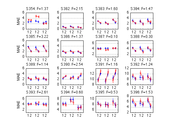
500: Contrasts for MAES02 [Developed on 2011-02-19]
Section 155 motivated the use of planned contrasts to maximize the power of the analysis of MAESpec01 data. Here we develop the MAESpec02 analog.
% Notation: Let us label the eight cells as follows:
%  * TU1 -- TRAIN, UPWARD direction at PRETEST -- assume MAE=M
%  * OU1 -- TRANSF (or Ortho), UPWARD dir. at PRETEST -- also MAE=M by symmetry
%  * TD1 -- TRAIN, DOWNWARD direction (aka Train180) at PRETEST -- assume MAE=M
%  * OD1 -- TRANSF (or Ortho), DOWNWARD dir. at PRETEST -- also MAE=M by symmetry
%  * TU2 -- TRAIN, UPWARD at POSTTEST -- *Change expected here!* -- (1+C)*M
%  * OU2 -- TRANSF (or Ortho), UPWARD at POSTEST -- assume MAE=M by specificity
%  * TD2 -- TRAIN, DOWNWARD at POSTTEST -- *Change possible here!* -- (1+D)*M
%  * OD2 -- TRANSF (or Ortho), DOWNWARD dir. at POSTTEST -- MAE=M by specif.
%
% Let's denote by C the *relative* size of the change (increase or decrease).
% Thus, the predicted MAE for TRAIN (and possibly TRAIN180) at POSTTEST is
% (1+C)*M, where M is the baseline MAE.  We'll do power analysis for a
% range of values C for the hypothetical change.  We are going to use the
% values defined in Section 155. They are stored in the hyp_change variable:

hyp_change

% Our 2x4 design has 7 df, which allows for 7 orthogonal contrasts, as follows:
%   DxR Cell          TU1 OU1 TD1 OD2 | TU2 OU2 TD2 OD2 | Mean
% ------------------------------------+-----------------+------
% 1 Main effect of Day -1  -1  -1  -1 |  +1  +1  +1  +1 |  0
% 2 TU1 <> OU1 @ PRE?  +2  -2   0   0 |   0   0   0   0 |  0  % expect no effect
% 3 TD1 <> OD1 @ PRE?   0   0  +2  -2 |   0   0   0   0 |  0  % expect no effect
% 4 TU2 <> OU2 @ POST?  0   0   0   0 |  +2  -2   0   0 |  0  % <-- Sic!
% 5 TD2 <> OD2 @ POST?  0   0   0   0 |   0   0  +2  -2 |  0  % <-- Sic!
% 6 UP <> DOWN maineff -1  -1  +1  +1 |  -1  -1  +1  +1 |  0
% 7(UP/DN) x Day inter -1  -1  +1  +1 |  +1  +1  -1  -1 |  0
% ------------------------------------+-----------------+------
%6a UP <> DOWN at PRE  -1  -1  +1  +1 |   0   0   0   0 |  0
%7a UP <> DOWN at POST  0   0   0   0 |  -1  -1  +1  +1 |  0
% ------------------------------------+-----------------+------
%   DxR Cell          TU1 OU1 TD1 OD2 | TU2 OU2 TD2 OD2 | Mean
%
% Contrasts 1-7 form a mutually orthogonal set. Alternatively, 6 & 7 can be
% replaced by 6a and 7a, which are also orthogonal to all the rest.
%
% Contrast 4 is a replication of the "Refdir at POST" contrast of MAESpec01,
% except that here there is STATIC only (whereas the analogous contrast in
% MAESpec02 averaged across STATIC and DYNAMIC).  This is useful because it
% will add 16 more subjects to the 11 subjects of MAESpec01.
%
% The new element introduced by the MAESpec02 experiment is the ability to
% test for Contrast 5 above -- are there MAE changes in the *opposite* of
% the trained direction relative to an orthogonal control at posttest?
%
% Contrasts 6 and 7 (or 6a and 7a) test whether MAE for upward directions
% is different from MAE for downward directions (and whether this interacts
% with Day).  Note that the trained vs. orthogonal distinction is ignored
% (to ensure that contrasts 6 and 7 are orthogonal to contrasts 2-5).

% We predict the following expected MAE durations for each cell:
% * TU1 = OU1 = M -- by symmetry
% * TD1 = TU1 = M -- assume the UP/DOWN distinction has no effect
% * TD1 = OD1 = M -- by symmetry
% * OU2 = OU1 = M -- assuming all perceptual learning is stimulus-specific
% * OD2 = OD1 = M
% * TU2 = (1+C)*M -- Predicted UPWARD effect with relative size C   <--Sic!
% * TD2 = (1+D)*M -- Predicted DOWNWARD effect with relative size D <--Sic!
%
% This yields the following expected values for each contrast:
% 'C1M' is a shorthand for '(1+C)*M'; 'D1M' is shorthand for '(1+D)*M'
%   DxR Cell          TU1 OU1 TD1 OD2 | TU2 OU2 TD2 OD2 | Mean
% ------------------------------------+-----------------+------
% 1 Main effect of Day -M  -M  -M  -M | +C1M +M +D1M +M |(C+D)*M/8 + criterion chng
% 2 TU1 <> OU1 @ PRE?  +2M -2M  0   0 |   0   0   0   0 |  0
% 3 TD1 <> OD1 @ PRE?   0   0  +2M -2M|   0   0   0   0 |  0
% 4 TU2 <> OU2 @ POST?  0   0   0   0 |+2C1M -2M  0   0 |+2C*M/8
% 5 TD2 <> OD2 @ POST?  0   0   0   0 |   0   0 +2D1M-2M|+2D*M/8
% 6 UP <> DOWN maineff -M  -M  +M  +M | -C1M -M +D1M +M |(D-C)*M/8 + Up/Dn anisotropy
% 7(UP/DN) x Day inter -M  -M  +M  +M | +C1M +M -D1M -M |(C-D)*M/8
% ------------------------------------+-----------------+------
%6a UP <> DOWN at PRE  -M  -M  +M  +M |   0   0   0   0 |  0       + Up/Dn anisotropy
%7a UP <> DOWN at POST  0   0   0   0 | -C1M -M +D1M +M |(D-C)*M/4
% ------------------------------------+-----------------+------
%   DxR Cell          TU1 OU1 TD1 OD2 | TU2 OU2 TD2 OD2 | Mean
% The hyp_psy variable calculated in Section 550 below must implement
% the above table.
%
% Technical note: The formulas normalize by the sum of squared contrast coefs,
% so the tables above should have used +-1/2 for the 4-term contrasts,
% +-1/sqrt(2) for the 2-term contrasts, and +-1/2sqrt2 for the 8-term c's.
% The contrast coefs will be represented as column vectors of length 8 that
% operate on the row vector of cell means across the 8 conditions.

% The relative change in the DOWNWARD dimension is conceptually distinct
% from the relative change in the UPWARD dimension. That's why it is
% denoted 'D' (as distinguished from 'C') above.  We are not going to
% define a new Matlab variable however. We'll use hyp_change for both C and
% D.  Note that this amounts to the hypothesis that D=C.
hyp_change =

    0.0500    0.1000    0.1500    0.2000    0.2500    0.3000
510: Define contrast coefficients
contrasts2 = NaN(N_cells,7+2) ;
contrast_names2 = cell(1,7+2) ;

% 1 Main effect of Day -1  -1  -1  -1 |  +1  +1  +1  +1 |  0
%   DxR Cell          TU1 OU1 TD1 OD2 | TU2 OU2 TD2 OD2 | Mean
V2.Day = 1 ;
contrast_names2{V2.Day} = 'Day' ;
contrasts2(V2.pretest,V2.Day) = -1 ;
contrasts2(V2.posttest,V2.Day) = +1 ;

% 2 TU1 <> OU1 @ PRE?  +2  -2   0   0 |   0   0   0   0 |  0  % expect no effect
%   DxR Cell          TU1 OU1 TD1 OD2 | TU2 OU2 TD2 OD2 | Mean
V2.TU1_OU1_PRE = 2 ;
contrast_names2{V2.TU1_OU1_PRE} = 'TU1_OU1_PRE' ;
contrasts2(V2.pretest&V2.train,V2.TU1_OU1_PRE) = +1 ;
contrasts2(V2.pretest&V2.transf,V2.TU1_OU1_PRE) = -1 ;
contrasts2(V2.pretest&V2.down,V2.TU1_OU1_PRE) = 0 ;
contrasts2(V2.posttest,V2.TU1_OU1_PRE) = 0 ;

% 3 TD1 <> OD1 @ PRE?   0   0  +2  -2 |   0   0   0   0 |  0  % expect no effect
%   DxR Cell          TU1 OU1 TD1 OD2 | TU2 OU2 TD2 OD2 | Mean
V2.TD1_OD1_PRE = 3 ;
contrast_names2{V2.TD1_OD1_PRE} = 'TD1_OD1_PRE' ;
contrasts2(V2.pretest&V2.up,V2.TD1_OD1_PRE) = 0 ;
contrasts2(V2.pretest&V2.train180,V2.TD1_OD1_PRE) = +1 ;
contrasts2(V2.pretest&V2.transf180,V2.TD1_OD1_PRE) = -1 ;
contrasts2(V2.posttest,V2.TD1_OD1_PRE) = 0 ;

% 4 TU2 <> OU2 @ POST?  0   0   0   0 |  +2  -2   0   0 |  0  % <-- Sic!
%   DxR Cell          TU1 OU1 TD1 OD2 | TU2 OU2 TD2 OD2 | Mean
V2.TU2_OU2_POST = 4 ;
contrast_names2{V2.TU2_OU2_POST} = 'TU2_OU2_POST' ;
contrasts2(V2.pretest,V2.TU2_OU2_POST) = 0 ;
contrasts2(V2.posttest&V2.train,V2.TU2_OU2_POST) = +1 ;
contrasts2(V2.posttest&V2.transf,V2.TU2_OU2_POST) = -1 ;
contrasts2(V2.posttest&V2.down,V2.TU2_OU2_POST) = 0 ;

% 5 TD2 <> OD2 @ POST?  0   0   0   0 |   0   0  +2  -2 |  0  % <-- Sic!
%   DxR Cell          TU1 OU1 TD1 OD2 | TU2 OU2 TD2 OD2 | Mean
V2.TD2_OD2_POST = 5 ;
contrast_names2{V2.TD2_OD2_POST} = 'TD2_OD2_POST' ;
contrasts2(V2.pretest,V2.TD2_OD2_POST) = 0 ;
contrasts2(V2.posttest&V2.up,V2.TD2_OD2_POST) = 0 ;
contrasts2(V2.posttest&V2.train180,V2.TD2_OD2_POST) = +1 ;
contrasts2(V2.posttest&V2.transf180,V2.TD2_OD2_POST) = -1 ;

% 6 UP <> DOWN maineff -1  -1  +1  +1 |  -1  -1  +1  +1 |  0
%   DxR Cell          TU1 OU1 TD1 OD2 | TU2 OU2 TD2 OD2 | Mean
V2.Up_Down = 6 ;
contrast_names2{V2.Up_Down} = 'Up_Down' ;
contrasts2(V2.up,V2.Up_Down) = -1 ;
contrasts2(V2.down,V2.Up_Down) = +1 ;

% 7(UP/DN) x Day inter -1  -1  +1  +1 |  +1  +1  -1  -1 |  0
%   DxR Cell          TU1 OU1 TD1 OD2 | TU2 OU2 TD2 OD2 | Mean
V2.DxUD = 7 ;
contrast_names2{V2.DxUD} = 'DxUD' ;
contrasts2(V2.pretest&V2.up,V2.DxUD) = -1 ;
contrasts2(V2.pretest&V2.down,V2.DxUD) = +1 ;
contrasts2(V2.posttest&V2.up,V2.DxUD) = +1 ;
contrasts2(V2.posttest&V2.down,V2.DxUD) = -1 ;

% 8=6a UP <> DOWN at PRE  -1  -1  +1  +1 |   0   0   0   0 |  0
%      DxR Cell          TU1 OU1 TD1 OD2 | TU2 OU2 TD2 OD2 | Mean
V2.Up_Down_PRE = 8 ;
contrast_names2{V2.Up_Down_PRE} = 'Up_Down_PRE' ;
contrasts2(V2.pretest&V2.up,V2.Up_Down_PRE) = -1 ;
contrasts2(V2.pretest&V2.down,V2.Up_Down_PRE) = +1 ;
contrasts2(V2.posttest,V2.Up_Down_PRE) = 0 ;

% 9=7a UP <> DOWN at POST  0   0   0   0 |  -1  -1  +1  +1 |  0
%      DxR Cell          TU1 OU1 TD1 OD2 | TU2 OU2 TD2 OD2 | Mean
V2.Up_Down_POST = 9 ;
contrast_names2{V2.Up_Down_POST} = 'Up_Down_POST' ;
contrasts2(V2.pretest,V2.Up_Down_POST) = 0 ;
contrasts2(V2.posttest&V2.up,V2.Up_Down_POST) = -1 ;
contrasts2(V2.posttest&V2.down,V2.Up_Down_POST) = +1 ;

% Display the contrast names (and the coefs below)
contrast_names2

% Normalize to unit length
contrasts2 = normalize_coefs(contrasts2)
contrast_names2 =

  Columns 1 through 7

    'Day'    'TU1_OU1_PRE'    'TD1_OD1_PRE'    'TU2_OU2_POST'    'TD2_OD2_POST'    'Up_Down'    'DxUD'

  Columns 8 through 9

    'Up_Down_PRE'    'Up_Down_POST'


contrasts2 =

   -0.3536    0.7071         0         0         0   -0.3536   -0.3536   -0.5000         0
   -0.3536   -0.7071         0         0         0   -0.3536   -0.3536   -0.5000         0
   -0.3536         0    0.7071         0         0    0.3536    0.3536    0.5000         0
   -0.3536         0   -0.7071         0         0    0.3536    0.3536    0.5000         0
    0.3536         0         0    0.7071         0   -0.3536    0.3536         0   -0.5000
    0.3536         0         0   -0.7071         0   -0.3536    0.3536         0   -0.5000
    0.3536         0         0         0    0.7071    0.3536   -0.3536         0    0.5000
    0.3536         0         0         0   -0.7071    0.3536   -0.3536         0    0.5000
520: Calculate SS for the Contrasts, MAESpec02
Equation 4.5 in Keppel & Wickens (2004, p. 69). Also MS==SS because df=1. This section is based on the analogous MAESpec01 Section 162 above.
Each contrast is calculated twice. First from the complete MAE (with imputed missing values) -- as a sanity check with the ANOVA SS that too are calculated on the complete MAE. Second from the MAE_duration (with NaNs) -- free of imputation assumptions. All subsequent analyses use the second (nanmean) set of contrasts.
MAES02_psy_F = NaN(N_MAES02_sbj,length(contrast_names2)) ;
MAES02_psy_p = NaN(N_MAES02_sbj,length(contrast_names2)) ;
MAES02_psy_w2p = NaN(N_MAES02_sbj,length(contrast_names2)) ;
MAES02_psy_w2c = NaN(N_MAES02_sbj,length(contrast_names2)) ;

for k = 1:N_MAES02_sbj
    %- Retrieve the cell means of the original design
    M = D2(k).cell_nanmean_MAE ./ msec2sec ; % [N_cells x 1], w/ NaNs
    M0 = mean(D2(k).MAE) ./ msec2sec ;       % [N_cells x 1], no missing vals

    %- Augment the indiv_ANOVA structure
    st = D2(k).indiv_ANOVA ;
    st.contrast_names = contrast_names2 ;

    %- Calculate the "observed value psy_hat of each contrast"
    psy = M*contrasts2 ;       % [1x9], Eq.4.4
    psy0 = M0*contrasts2 ;     % [1x9], Eq.4.4
    st.psy_NaN = psy ;
    st.psy_noNaN = psy0 ;

    %- Convert each observed contrast into a sum of squares (Eq.4.5)
    % Note that the coefficients are already normalized.
    SS = N_reps_per_cell * psy.^2 ;
    SS0 = N_reps_per_cell * psy0.^2 ;
    st.SS_psy_NaN = SS ;
    st.SS_psy_noNaN = SS0 ;

    %- Sanity check: SS0(V2.Day) should match indiv_ANOVA.SS('D'=1)
    assert(eq0(SS0(V2.Day) - st.SS(1))) ;

    %- Sanity check: Additivity of the two alternative partitions of c6+c7
    assert(eq0((SS0(V2.Up_Down)+SS0(V2.DxUD)) - ...          % w/o NaNs
               (SS0(V2.Up_Down_PRE)+SS0(V2.Up_Down_POST)) )) ;
    assert(eq0((SS(V2.Up_Down)+SS(V2.DxUD)) - ...            % w/ NaNs
               (SS(V2.Up_Down_PRE)+SS(V2.Up_Down_POST)) )) ;

    %- Calculate F ratios
    % All these contrasts have df=1 and hence MS=SS. All use a common
    % error term -- MS_err from the overall analysis (Eq 4.6).
    F = SS ./ st.MS_err ;
    F0 = SS0 ./ st.MS_err ;
    st.F_psy_NaN = F ;
    st.t_psy_NaN = sqrt(F) ;
    st.F_psy_noNaN = F0 ;
    st.t_psy_noNaN = sqrt(F0) ;
    MAES02_psy_F(k,:) = F ;

    %- Calculate significance
    st.p_psy_NaN = 1-fcdf(F,1,st.adjusted_df_err) ;
    st.p_psy_noNaN = 1-fcdf(F0,1,st.adjusted_df_err) ;
    MAES02_psy_p(k,:) = st.p_psy_noNaN ;

    %- Calculate partial and complete omega-squared (Eqs. 21.7 & 21.8)
    N = st.df(end)+1 ;  % 168 = total # of scores
    w2 = 1 .* (F-1) ;   % df=1
    w2 = max(0,w2) ;  % F values < 1.0 are entirely due to sampling error.
    st.partial_omega2_psy = w2./(w2+N) ;        % Eq. 21.7
    st.complete_omega2_psy = w2./(sum(w2)+N) ;  % Eq. 21.9
    MAES02_psy_w2p(k,:) = st.partial_omega2_psy ;
    MAES02_psy_w2c(k,:) = st.complete_omega2_psy ;

    %- Store and move on
    D2(k).indiv_ANOVA = st ;
end
clearvars k M M0 st psy psy0 SS SS0 F F0 w2 N ;
530: Report the contrast-based test results, MAESpec02
This section is based on the analogous MAESpec01 Section 163 above.
Note: The F ratio for Dayis based on nanmeans and hence differs slightly from the one reported in section 402 above. Arguably, the one reported here should take precedence because it does not depend on assumptions about filled-in missing values. In this scheme, the imputed values only influence the MS_err (but not adjusted_df_err).
disp(contrast_names2)
MAES02_psy_F

fprintf('Distribution of contrast-based Fs, %d MAES01 Ss:',N_MAES02_sbj) ;
describe(MAES02_psy_F,contrast_names2) ;
fprintf('Critical F(1,160) = %.2f (p<.05)\n',finv(.95,1,160)) ;

fprintf('\nCorresponding t values:') ;
describe(sqrt(MAES02_psy_F),contrast_names2) ;

fprintf('\nCorresponding p values:') ;
describe(MAES02_psy_p,contrast_names2) ;

fprintf('\nCorresponding PARTIAL omega^2 [%%] -- Eq.21.7 in Keppel&Wickens:') ;
describe(MAES02_psy_w2p.*100,contrast_names2) ;

fprintf('\nCorresponding COMPLETE omega^2 [%%] -- Eq.21.9') ;
describe(MAES02_psy_w2c.*100,contrast_names2) ;

% Some quick comments:
% * Day (contrast 1) has a robust effect. It is significant for the
%   majority of the subjects. This confirms the group-level plot (Sect.430)
%   showing longer MAEs at pretest rather than posttest.  Interestingly,
%   this replicates the direction of the overall main effect of Day in the
%   MAESpec01 experiment (Sect.180). However, the relevant MAES01 comparison
%   is for the STATIC subgroup, and there the pretest MAE is *lower* than
%   the posttest MAE (plot in Section 180, middle tetrade of points).
%
% * UP-vs-DOWN (contrast 6) also is significant for the majority of the Ss.
%   The upward motion elicits a slightly (but significantly?) longer MAE
%   than the downward motion, irrespective of day.  (Except for a few
%   subjects, who do show a UD-by-Day interaction.)
%
% * Our main question, however, is about TRAIN vs TRANSF at posttest.
%   This is tested separately for upward (c4) and downward (c5) motion.
%   Sections 533 and 536 inspect these two contrasts in detail.
  Columns 1 through 7

    'Day'    'TU1_OU1_PRE'    'TD1_OD1_PRE'    'TU2_OU2_POST'    'TD2_OD2_POST'    'Up_Down'    'DxUD'

  Columns 8 through 9

    'Up_Down_PRE'    'Up_Down_POST'


MAES02_psy_F =

    0.0479   27.2123    0.3479   32.7554    3.4168   81.9276    3.1935   58.7358   26.3854
   46.6684    5.6247    0.6744    0.1046    0.0008    6.9556    4.0858   10.8516    0.1897
   45.8579    1.1700    0.0861    0.0730    3.1215   52.6570    2.8112   39.9008   15.5674
   20.1761    0.0120    2.5001    0.2133    1.6588    4.8474    0.2420    1.4616    3.6278
  106.7694    8.8265    0.1298    0.1469    0.9813   14.1545    5.3880   18.5042    1.0383
   31.3309    1.4277    0.3004    2.4978    0.0179    2.8069    0.0229    1.6687    1.1612
    0.0024    6.1733    0.1018    3.7348    0.0382    4.8442    0.0064    2.6017    2.2490
   39.7226    2.8683    0.1611    1.7627    0.5271    3.0166    0.7918    0.3587    3.4497
   10.4629    1.3852    0.3573    1.9673    0.0605    0.7489    0.0239    0.5201    0.2527
   20.0810    0.7383    1.4625    1.8011    4.8625    8.9671    4.7031    0.3410   13.3292
   59.1216    0.0174    1.2392    1.2488    1.7276    2.1168    0.0730    1.4881    0.7018
    8.4092    5.1346    0.5804    0.0207    0.2231    2.3002    0.0000    1.1555    1.1448
    0.0006    2.5873    0.7423    4.6841    2.1602    3.9225    0.5325    0.7823    3.6728
    0.0018    0.5018    0.1869    4.1672    0.0094   64.2023    0.8527   39.9265   25.1285
    3.2307    0.0035    0.5294    0.0866    0.0144    1.3246    1.0053    2.3189    0.0110
   22.1816    1.8386    0.1951    0.2690    0.4703    0.0405    4.3602    2.6208    1.7799

Distribution of contrast-based Fs, 16 MAES01 Ss:
    Mean  Std.dev       Min     Q25  Median     Q75     Max
------------------------------------------------------------
  25.879   28.882      0.00    1.64   20.13   42.79  106.77  Day
   4.095    6.686      0.00    0.62    1.63    5.38   27.21  TU1_OU1_PRE
   0.600    0.646      0.09    0.17    0.35    0.71    2.50  TD1_OD1_PRE
   3.471    7.965      0.02    0.13    1.51    3.12   32.76  TU2_OU2_POST
   1.206    1.499      0.00    0.03    0.50    1.94    4.86  TD2_OD2_POST
  15.927   25.779      0.04    2.21    4.38   11.56   81.93  Up_Down
   1.756    1.972      0.00    0.05    0.82    3.64    5.39  DxUD
  11.452   18.306      0.34    0.97    1.99   14.68   58.74  Up_Down_PRE
   6.231    8.861      0.01    0.87    2.01    8.50   26.39  Up_Down_POST
------------------------------------------------------------
   7.846   11.177      0.06    0.74    3.70   10.26   38.50
Critical F(1,160) = 3.90 (p<.05)

Corresponding t values:
    Mean  Std.dev       Min     Q25  Median     Q75     Max
------------------------------------------------------------
   4.092    3.121      0.02    1.01    4.49    6.54   10.33  Day
   1.581    1.305      0.06    0.78    1.28    2.32    5.22  TU1_OU1_PRE
   0.691    0.361      0.29    0.42    0.59    0.84    1.58  TD1_OD1_PRE
   1.314    1.364      0.14    0.35    1.22    1.76    5.72  TU2_OU2_POST
   0.849    0.719      0.03    0.16    0.71    1.39    2.21  TD2_OD2_POST
   3.044    2.666      0.20    1.49    2.09    3.38    9.05  Up_Down
   1.048    0.838      0.00    0.21    0.91    1.90    2.32  DxUD
   2.515    2.339      0.58    0.98    1.41    3.80    7.66  Up_Down_PRE
   1.957    1.601      0.10    0.93    1.42    2.78    5.14  Up_Down_POST
------------------------------------------------------------
   1.899    1.590      0.16    0.70    1.57    2.75    5.47

Corresponding p values:
    Mean  Std.dev       Min     Q25  Median     Q75     Max
------------------------------------------------------------
   0.239    0.416      0.00    0.00    0.00    0.45    0.98  Day
   0.299    0.339      0.00    0.02    0.19    0.44    0.95  TU1_OU1_PRE
   0.516    0.197      0.12    0.39    0.55    0.68    0.77  TD1_OD1_PRE
   0.380    0.322      0.00    0.09    0.23    0.69    0.89  TU2_OU2_POST
   0.501    0.357      0.03    0.17    0.48    0.87    0.98  TD2_OD2_POST
   0.134    0.230      0.00    0.00    0.04    0.14    0.89  Up_Down
   0.430    0.368      0.02    0.06    0.37    0.83    0.99  DxUD
   0.204    0.197      0.00    0.00    0.16    0.33    0.56  Up_Down_PRE
   0.253    0.289      0.00    0.03    0.16    0.36    0.99  Up_Down_POST
------------------------------------------------------------
   0.329    0.302      0.02    0.08    0.24    0.53    0.89

Corresponding PARTIAL omega^2 [%] -- Eq.21.7 in Keppel&Wickens:
    Mean  Std.dev       Min     Q25  Median     Q75     Max
------------------------------------------------------------
  11.457   11.317      0.00    0.66   10.22   19.90   38.63  Day
   1.821    3.399      0.00    0.00    0.38    2.54   13.50  TU1_OU1_PRE
   0.081    0.227      0.00    0.00    0.00    0.00    0.89  TD1_OD1_PRE
   1.502    3.906      0.00    0.00    0.30    1.24   15.90  TU2_OU2_POST
   0.401    0.676      0.00    0.00    0.00    0.56    2.25  TD2_OD2_POST
   6.790   10.712      0.00    0.71    1.97    5.89   32.51  Up_Down
   0.677    0.956      0.00    0.00    0.00    1.55    2.55  DxUD
   5.119    8.425      0.00    0.05    0.59    7.49   25.58  Up_Down_PRE
   2.903    4.570      0.00    0.01    0.60    4.20   13.13  Up_Down_POST
------------------------------------------------------------
   3.417    4.910      0.00    0.16    1.56    4.82   16.10

Corresponding COMPLETE omega^2 [%] -- Eq.21.9
    Mean  Std.dev       Min     Q25  Median     Q75     Max
------------------------------------------------------------
  10.320   10.030      0.00    0.65    9.30   16.53   33.40  Day
   1.178    1.768      0.00    0.00    0.32    2.12    6.64  TU1_OU1_PRE
   0.068    0.195      0.00    0.00    0.00    0.00    0.76  TD1_OD1_PRE
   0.923    1.997      0.00    0.00    0.23    0.90    8.05  TU2_OU2_POST
   0.272    0.479      0.00    0.00    0.00    0.47    1.79  TD2_OD2_POST
   4.816    7.343      0.00    0.60    1.79    3.92   21.25  Up_Down
   0.452    0.675      0.00    0.00    0.00    0.93    1.72  DxUD
   3.301    5.209      0.00    0.04    0.55    4.84   14.63  Up_Down_PRE
   1.875    2.707      0.00    0.01    0.54    3.00    8.11  Up_Down_POST
------------------------------------------------------------
   2.578    3.378      0.00    0.14    1.41    3.64   10.71
531: How many effects are significant at various alpha levels?
See Section 404 for the analogous summary of the conventional partitioning of the same variance. See Section 164 for the MAESpec01 analog. Added 2011-03-19, AAP.
alphas = [.001 .005 .01 .05 .10] ;

contrast_names2     % print column labels
MAES02_psy_p        % print the p values for each effect and each sbj

for k = 1:length(alphas)
    fprintf('p<%.3f -->  %s \n',alphas(k),mat2str(sum(MAES02_psy_p<alphas(k)))) ;
end

% We verify the result from Section 404 that that 11 of 16 Ss have a
% significant effect of Day (at p<.05).
% There are other patterns here, but they will not end up in the published
% paper because the plan is to use the conventional partition for Exp 2.

clearvars k alphas ;
contrast_names2 =

  Columns 1 through 7

    'Day'    'TU1_OU1_PRE'    'TD1_OD1_PRE'    'TU2_OU2_POST'    'TD2_OD2_POST'    'Up_Down'    'DxUD'

  Columns 8 through 9

    'Up_Down_PRE'    'Up_Down_POST'


MAES02_psy_p =

    0.8271    0.0000    0.5561    0.0000    0.0664    0.0000    0.0758    0.0000    0.0000
    0.0000    0.0190    0.3909    0.7468    0.9772    0.0098    0.0471    0.0014    0.6638
    0.0000    0.2810    0.7696    0.7874    0.0792    0.0000    0.0956    0.0000    0.0001
    0.0000    0.9130    0.1158    0.6448    0.1996    0.0291    0.6234    0.2285    0.0586
         0    0.0034    0.7191    0.7021    0.3234    0.0002    0.0215    0.0000    0.3098
    0.0000    0.2339    0.5844    0.1160    0.8938    0.0958    0.8798    0.1983    0.2828
    0.9608    0.0140    0.7501    0.0551    0.8454    0.0292    0.9362    0.1087    0.1357
    0.0000    0.0923    0.6887    0.1862    0.4689    0.0843    0.3749    0.5501    0.0651
    0.0015    0.2410    0.5509    0.1604    0.8061    0.3860    0.8805    0.4719    0.6121
    0.0000    0.3915    0.2283    0.1815    0.0289    0.0032    0.0316    0.5601    0.0004
    0.0000    0.8952    0.2673    0.2655    0.1966    0.1501    0.7806    0.2243    0.4104
    0.0041    0.0235    0.4488    0.8859    0.6373    0.1290    0.9898    0.2783    0.2863
    0.9809    0.1097    0.3902    0.0319    0.1436    0.0494    0.4666    0.3778    0.0571
    0.9659    0.4798    0.6661    0.0429    0.9228    0.0000    0.3572    0.0000    0.0000
    0.0815    0.9526    0.4680    0.6716    0.9385    0.2888    0.2778    0.1298    0.9861
    0.0000    0.1408    0.6593    0.6048    0.4938    0.8895    0.0444    0.1278    0.1841

p<0.001 -->  [9 1 0 1 0 4 0 4 4]
p<0.005 -->  [11 2 0 1 0 5 0 5 4]
p<0.010 -->  [11 2 0 1 0 6 0 5 4]
p<0.050 -->  [11 5 0 3 1 9 4 5 4]
p<0.100 -->  [12 6 0 4 3 11 6 5 7]
533: Identify the subjects for whom TU2_OU2_POST is significant
%- Plot p(TU2_OU2_POST) vs p(TU1_OU1_PRE)
clf
plot(MAES02_psy_p(:,V2.TU1_OU1_PRE),MAES02_psy_p(:,V2.TU2_OU2_POST),'o') ;
axis([-.05 1.05 -.05 1.05]) ; axis square ; grid on ;
set(gca,'XTick',xtick_p,'YTick',xtick_p) ;
xlabel('p for Train<>Transf at PRETEST, UPWARD') ;
ylabel('p at POSTTEST') ;
title('MAES02: TRAIN vs TRANSF, UPWARD') ;

%- Now find those whose psy_p < 0.05
idx = find(MAES02_psy_p(:,V2.TU2_OU2_POST)<.05)'
[D2(idx).sbj]
MAES02_psy_p(idx,[V2.TU1_OU1_PRE V2.TU2_OU2_POST])

% Conclusion:
% Three of the 16 subjects show significant differences b/n TRAIN and
% TRANSF (upward motion) at POSTTEST.  These are subjects #354, 393, and
% 394 (stored at indices 1, 13, and 14, respectively).
% A look at the individual plots in Section 440 above convinces us,
% however, that the first of those -- subject 354 (idx=1) -- actually just
% reports a stronger MAE for the TRANSF direction *on both days*.  Thus,
% sbj 354 does not really show the interaction we are looking for.
%
% This highlights the fact that our contrast TU2_OU2_POST has a high
% statistical power in part because it depends on the *assumption* that the
% TRAIN and TRANSF directions yield equivalent MAEs prior to training. When
% this assumption is violated, TU2_OU2_POST becomes significant because it
% does not compare about the PRETEST baseline (which would lose power).
%
% In light of all this, I don't think it's cheating if we count only *two*
% subjects -- 393 and 394 -- as showing significant evidence in favor of
% the representation modification hypothesis. We should keep in mind that
% none of these 3 subjects shows significant Day-by-Refidir interaction
% overall (as reported in Section 402 above).
%
% To summarize the final tally along the UPWARD reference direction:
% 2 out of 16 subjects show significant differences b/n TRAIN and TRANSFER
% motion directions at posttest.
idx =

     1    13    14


ans =

   354   393   394


ans =

    0.0000    0.0000
    0.1097    0.0319
    0.4798    0.0429
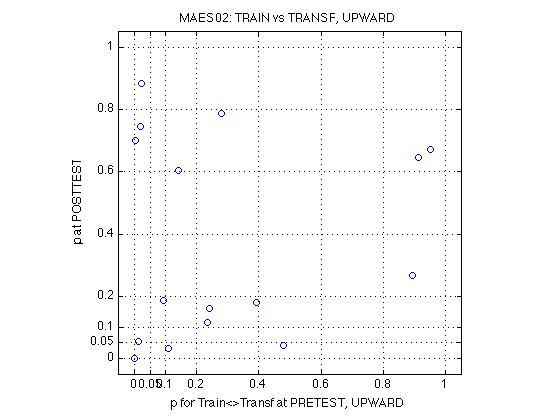
536: Analogously for TD2_OD2_POST
%- Plot p(TD2_OD2_POST) vs p(TD1_OD1_PRE)
clf
plot(MAES02_psy_p(:,V2.TD1_OD1_PRE),MAES02_psy_p(:,V2.TD2_OD2_POST),'o') ;
axis([-.05 1.05 -.05 1.05]) ; axis square ; grid on ;
set(gca,'XTick',xtick_p,'YTick',xtick_p) ;
xlabel('p for Train<>Transf at PRETEST, DOWNWARD') ;
ylabel('p at POSTTEST') ;
title('MAES02: TRAIN vs TRANSF, DOWNWARD') ;

%- Now find those whose psy_p < 0.05
idx = find(MAES02_psy_p(:,V2.TD2_OD2_POST)<.05)'
[D2(idx).sbj]
MAES02_psy_p(idx,[V2.TD1_OD1_PRE V2.TD2_OD2_POST])

% Conclusion:
% Only one of the 16 subjects (#390, idx=10) shows a significant difference
% b/n TRAIN and TRANSF in the *opposite* (downward) direction of motion at
% POSTTEST.
idx =

    10


ans =

   390


ans =

    0.2283    0.0289
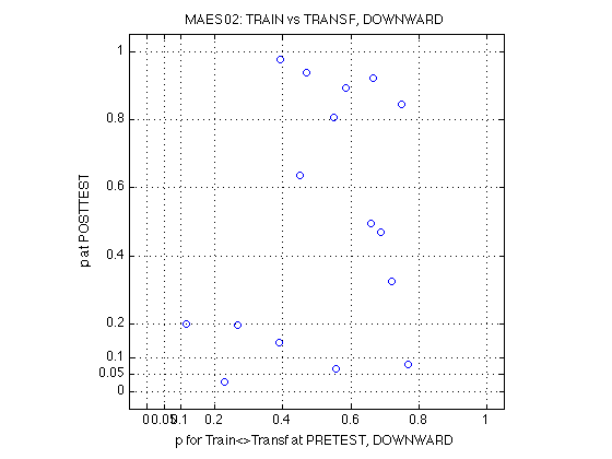
550: Power analysis for the individual MAES02 ANOVAs
This section is based on the analogous MAESpec01 Sections 165-168 above.
The power to reject the null hypothesis (all means=gradmean) must be calculated with respect to a concrete alternative hypothesis. This is where the frequentist framework acquires a Bayesian flavor.
Our alternative hyp is specified as a one-parameter family, as described in Section 500 above. The parameter in question is the hypothesized change in the MAE duration for the trained direction at posttest, relative (that is, divided by) the average MAE. We're going to calculate the power for the values in HYP_CHANGE.
pwr2.contrast_names = contrast_names2 ;     % superseded below
pwr2.contrasts = contrasts2 ;
pwr2.hyp_change = hyp_change ;      % [1x6]
N_hyp_change = length(hyp_change) ;

%- Postulate population means for each of these 6 alternative hypotheses
% From Sect.500 above: Expected MAE durations for each cell:
% * TU1 = OU1 = M -- by symmetry
% * TD1 = TU1 = M -- assume the UP/DOWN distinction has no effect
% * TD1 = OD1 = M -- by symmetry
% * OU2 = OU1 = M -- assuming all perceptual learning is stimulus-specific
% * OD2 = OD1 = M
% * TU2 = (1+C)*M -- Predicted UPWARD effect with relative size C   <--Sic!
% * TD2 = (1+D)*M -- Predicted DOWNWARD effect with relative size D <--Sic!
%
% As stated earlier, we are going to use the same hyp_change values for
% both C and D, although they are conceptually distinct.  This is not a
% problem because the respective contrasts will be evaluated separately.

hyp_MAE_means = NaN(N_hyp_change,N_cells) ;    % [6x8]

hyp_MAE_means(:,V2.pretest) = 1 ;              % = mean MAE
hyp_MAE_means(:,V2.posttest&V2.transf) = 1 ;
hyp_MAE_means(:,V2.posttest&V2.transf180) = 1 ;
hyp_MAE_means(:,V2.posttest&V2.train) = 1+hyp_change' ;
hyp_MAE_means(:,V2.posttest&V2.train180) = 1+hyp_change'
pwr2.hyp_MAE_means = hyp_MAE_means ;

%- Calculate the hypothesized contrast values (Eq. 4.4)
% These values should agree with the corresponding table in the comments to
% Section 500 above.
hyp_psy = hyp_MAE_means * contrasts2        % [6x9] = [6x8]*[8x9]
pwr2.hyp_psy = hyp_psy ;

%- Calculate the variance sigma^2_psy for each contrast (Eq.8.13)
% (The coefficients are already normalized.)
hyp_s2_psy = (hyp_psy.^2)'/2
pwr2.hyp_s2_psy = hyp_s2_psy ;
hyp_MAE_means =

    1.0000    1.0000    1.0000    1.0000    1.0500    1.0000    1.0500    1.0000
    1.0000    1.0000    1.0000    1.0000    1.1000    1.0000    1.1000    1.0000
    1.0000    1.0000    1.0000    1.0000    1.1500    1.0000    1.1500    1.0000
    1.0000    1.0000    1.0000    1.0000    1.2000    1.0000    1.2000    1.0000
    1.0000    1.0000    1.0000    1.0000    1.2500    1.0000    1.2500    1.0000
    1.0000    1.0000    1.0000    1.0000    1.3000    1.0000    1.3000    1.0000


hyp_psy =

    0.0354         0         0    0.0354    0.0354         0         0         0         0
    0.0707         0         0    0.0707    0.0707         0         0         0         0
    0.1061         0         0    0.1061    0.1061         0         0         0         0
    0.1414         0         0    0.1414    0.1414         0         0         0         0
    0.1768         0         0    0.1768    0.1768         0         0         0         0
    0.2121         0         0    0.2121    0.2121         0         0         0         0


hyp_s2_psy =

    0.0006    0.0025    0.0056    0.0100    0.0156    0.0225
         0         0         0         0         0         0
         0         0         0         0         0         0
    0.0006    0.0025    0.0056    0.0100    0.0156    0.0225
    0.0006    0.0025    0.0056    0.0100    0.0156    0.0225
         0         0         0         0         0         0
         0         0         0         0         0         0
         0         0         0         0         0         0
         0         0         0         0         0         0
560: Add the conventional 4-level factors to the mix.
The sigma2 for Refdir factor (with 4 levels) can be calculated according to Eq. 8.9 on p. 163 in Keppel & Wickens.
Note that here we do assume that the parameters C and D are equal. That is, that the change in the ANTI-trained direction will be present and equal to that in the trained direction. This will generate stronger effects across all 4 Refdirs and thus predicts greater power than would be the case if only the upward trained direction was changed. On the other hand, it does make theoretical sense to expect that the anti-trained direction may be affected as well. After all, the perceived direction of the aftereffect is opposite to the direction of the inducer stimulus.
%- First, we need to average Day out of the picture
hyp_MAE_means2 = (hyp_MAE_means(:,V2.pretest)+hyp_MAE_means(:,V2.posttest))./2
pwr2.hyp_MAE_means2 = hyp_MAE_means2 ;

%- Deviations alpha_j of the group mean for each Refdir from the grand mean:
hyp_MAE_Refdir_deviations = repmat(mean(hyp_MAE_means2,2),1,4) ;
hyp_MAE_Refdir_deviations = hyp_MAE_means2 - hyp_MAE_Refdir_deviations
pwr2.hyp_MAE_Refdir_deviations = hyp_MAE_Refdir_deviations ;

%- By definition, the variance is just the mean squared deviation (Eq.8.9):
% Note that this is the sum-of-squares (SS) rather than *mean* SS (Eq.4.1).
% This clarification is relevant because Refdir has df=3 and thus MS=SS/3.
hyp_s2_Refdir = mean(hyp_MAE_Refdir_deviations.^2,2)'
pwr2.hyp_s2_Refdir = hyp_s2_Refdir ;


%- We'll calculate the variance of the Refdir-by-Day interaction by
% subtracting the Refdir SS (which has df=3) from the sum SS of contrasts
% number 2 through 7 above (that is, the total SS except that for the main
% effect of Day, which was averaged out above).
SS = sum(hyp_s2_psy(V2.TU1_OU1_PRE : V2.DxUD, :))
hyp_s2_RxD = SS - hyp_s2_Refdir
pwr2.hyp_s2_RxD = hyp_s2_RxD ;

% Note that under these assumptions the RxD interaction has a stronger
% effect (and hence more power) than the TU2_OU2_POST contrast above.
% Once again, this is because it assumes that *both* the upward and the
% downward trained direction will change.
%
% We could calculate an alternative set of Refdir expected MAEs, assuming
% that *only* the upward TRAIN direction will change, whereas all downward
% directions remain unchanged.  This will have the same SS as TU2_OU2_POST
% but df=3 rather than 1 and thus less power.  Thus, this model is
% dominated by the TU2_OU2_POST contrast which we have already.

%- Define a new variable "augmented" hyp_s2_psy to streamline the rest of
% the power-related calculations
hyp_s2_psy2 = [hyp_s2_psy ; hyp_s2_Refdir ; hyp_s2_RxD]
pwr2.hyp_s2_psy2 = hyp_s2_psy2 ;

V2.Refdir = V2.Up_Down_POST + 1 ;  % = 10
V2.DxR = V2.Refdir + 1 ;           % = 11

contrast_names2a = cat(2,contrast_names2,{'Refdir','DxR'})
pwr2.contrast_names = contrast_names2a ;  % overwriting the value set above

clearvars hyp_s2_psy hyp_MAE_means2 hyp_MAE_Refdir_deviations hyp_s2_Refdir SS
hyp_MAE_means2 =

    1.0250    1.0000    1.0250    1.0000
    1.0500    1.0000    1.0500    1.0000
    1.0750    1.0000    1.0750    1.0000
    1.1000    1.0000    1.1000    1.0000
    1.1250    1.0000    1.1250    1.0000
    1.1500    1.0000    1.1500    1.0000


hyp_MAE_Refdir_deviations =

    0.0125   -0.0125    0.0125   -0.0125
    0.0250   -0.0250    0.0250   -0.0250
    0.0375   -0.0375    0.0375   -0.0375
    0.0500   -0.0500    0.0500   -0.0500
    0.0625   -0.0625    0.0625   -0.0625
    0.0750   -0.0750    0.0750   -0.0750


hyp_s2_Refdir =

    0.0002    0.0006    0.0014    0.0025    0.0039    0.0056


SS =

    0.0013    0.0050    0.0112    0.0200    0.0312    0.0450


hyp_s2_RxD =

    0.0011    0.0044    0.0098    0.0175    0.0273    0.0394


hyp_s2_psy2 =

    0.0006    0.0025    0.0056    0.0100    0.0156    0.0225
         0         0         0         0         0         0
         0         0         0         0         0         0
    0.0006    0.0025    0.0056    0.0100    0.0156    0.0225
    0.0006    0.0025    0.0056    0.0100    0.0156    0.0225
         0         0         0         0         0         0
         0         0         0         0         0         0
         0         0         0         0         0         0
         0         0         0         0         0         0
    0.0002    0.0006    0.0014    0.0025    0.0039    0.0056
    0.0011    0.0044    0.0098    0.0175    0.0273    0.0394


contrast_names2a =

  Columns 1 through 7

    'Day'    'TU1_OU1_PRE'    'TD1_OD1_PRE'    'TU2_OU2_POST'    'TD2_OD2_POST'    'Up_Down'    'DxUD'

  Columns 8 through 11

    'Up_Down_PRE'    'Up_Down_POST'    'Refdir'    'DxR'
570: Power analysis, continued from Section 550
%- Take the median, normalized MS_err calculated in Section 410 above:
pwr2.median_norm_MS_err = median(mean_MAE_by_sbj.MAES02_MS_err(:,2)) ;

%- Calculate the partial effect size (omega^2) for each contrast (Eq.8.15)
w2p = pwr2.hyp_s2_psy2 ./ (pwr2.hyp_s2_psy2+pwr2.median_norm_MS_err)
pwr2.partial_omega2 = w2p ;

%- Calculate the "noncentrality parameter phi" (Eq. 8.19)
phi = sqrt((N_reps_per_cell.*w2p)./(1-w2p))
pwr2.phi = phi ;

%- Read off the power from the power chart defined in Section 166
power = interp1(power_chart.phi,power_chart.power,pwr2.phi)
pwr2.power = power ;


%- Pull out the two most relevant tests
% As TD2_OD2_POST has exactly the same power as TU2_OU2_POST, it need not
% be highlighted in a separate field.
pwr2.power_TU1_OU1_POST = power(V2.TU2_OU2_POST,:) ;
pwr2.power_DxR_strong = power(V2.DxR,:) ;     % see comments above

% Let's define a weaker version of DxR halfway between the strong version
% and TU2_OU2_POST.  This represents some compromise between asserting that
% *both* upward and downward MAEs will change (as DxR_strong asserts), on
% one hand, and asserting that *either* upward *or* downward (but not both)
% can change (as TU2_OU2_POST and TD2_OD2_POST assert, separately).
pwr2.power_DxR_weak = (pwr2.power_TU1_OU1_POST + pwr2.power_DxR_strong)./2

clearvars N_hyp_change hyp_MAE_means hyp_psy hyp_s2_psy2 w2p phi power ;
w2p =

    0.0055    0.0216    0.0474    0.0813    0.1215    0.1660
         0         0         0         0         0         0
         0         0         0         0         0         0
    0.0055    0.0216    0.0474    0.0813    0.1215    0.1660
    0.0055    0.0216    0.0474    0.0813    0.1215    0.1660
         0         0         0         0         0         0
         0         0         0         0         0         0
         0         0         0         0         0         0
         0         0         0         0         0         0
    0.0014    0.0055    0.0123    0.0216    0.0334    0.0474
    0.0096    0.0373    0.0801    0.1341    0.1948    0.2584


phi =

    0.3408    0.6816    1.0224    1.3632    1.7040    2.0448
         0         0         0         0         0         0
         0         0         0         0         0         0
    0.3408    0.6816    1.0224    1.3632    1.7040    2.0448
    0.3408    0.6816    1.0224    1.3632    1.7040    2.0448
         0         0         0         0         0         0
         0         0         0         0         0         0
         0         0         0         0         0         0
         0         0         0         0         0         0
    0.1704    0.3408    0.5112    0.6816    0.8520    1.0224
    0.4508    0.9017    1.3525    1.8033    2.2542    2.7050


power =

    0.0741    0.1586    0.3012    0.4798    0.6772    0.8234
    0.0500    0.0500    0.0500    0.0500    0.0500    0.0500
    0.0500    0.0500    0.0500    0.0500    0.0500    0.0500
    0.0741    0.1586    0.3012    0.4798    0.6772    0.8234
    0.0741    0.1586    0.3012    0.4798    0.6772    0.8234
    0.0500    0.0500    0.0500    0.0500    0.0500    0.0500
    0.0500    0.0500    0.0500    0.0500    0.0500    0.0500
    0.0500    0.0500    0.0500    0.0500    0.0500    0.0500
    0.0500    0.0500    0.0500    0.0500    0.0500    0.0500
    0.0585    0.0741    0.1078    0.1586    0.2234    0.3012
    0.0927    0.2458    0.4739    0.7313    0.8835    0.9705


pwr2 =

               contrast_names: {1x11 cell}
                    contrasts: [8x9 double]
                   hyp_change: [0.0500 0.1000 0.1500 0.2000 0.2500 0.3000]
                hyp_MAE_means: [6x8 double]
                      hyp_psy: [6x9 double]
                   hyp_s2_psy: [9x6 double]
               hyp_MAE_means2: [6x4 double]
    hyp_MAE_Refdir_deviations: [6x4 double]
                hyp_s2_Refdir: [1.5625e-04 6.2500e-04 0.0014 0.0025 0.0039 0.0056]
                   hyp_s2_RxD: [0.0011 0.0044 0.0098 0.0175 0.0273 0.0394]
                  hyp_s2_psy2: [11x6 double]
           median_norm_MS_err: 0.1130
               partial_omega2: [11x6 double]
                          phi: [11x6 double]
                        power: [11x6 double]
           power_TU1_OU1_POST: [0.0741 0.1586 0.3012 0.4798 0.6772 0.8234]
             power_DxR_strong: [0.0927 0.2458 0.4739 0.7313 0.8835 0.9705]
               power_DxR_weak: [0.0834 0.2022 0.3875 0.6055 0.7804 0.8970]
580: Family-wise power across the 16 individual MAES02 tests
This section is based on the analogous MAESpec01 Section 170 above.
%- Probability of 2 out of N outcomes
% The functions p_0ofN and p_1ofN were defined in Section 170 above:
% p_0ofN = @(p,N) ((1-p).^N) ;
% p_1ofN = @(p,N) (N.*p.*(1-p).^(N-1)) ;
%
% Here we need p_2ofN because 2 subjects got signif TU2_OU2_POST.
% The general formula for "k of N" is described by the terms of the
% binomial distribution. See Chapter VI in Feller (1957, vol.1, Eq.2.1, p.137).
% The Matlab function nchoosek calculates the binomial coefficients.
% See also Eq. 4.3 in Feller. We need nchoosek(16,2) = 120 = 16*(16-1)/2
p_2ofN = @(p,N) ((N*(N-1)/2) .* p.^2 .* (1-p).^(N-2)) ;

%-- 0 of 16
pwr2.comment_0of16 = 'When the outcome is 0 hits out of 16 individual tests' ;
pwr2.prob_0of16_TU1_OU1_POST = p_0ofN(pwr2.power_TU1_OU1_POST,N_MAES02_sbj) ;
pwr2.prob_0of16_DxR_strong = p_0ofN(pwr2.power_DxR_strong,N_MAES02_sbj) ;
pwr2.prob_0of16_DxR_weak = p_0ofN(pwr2.power_DxR_weak,N_MAES02_sbj) ;

%- Probability of making 0 type-I errors in 16 tests if the null hyp is true
pwr2.prob_0of16_null = p_0ofN(.05,N_MAES02_sbj) ;    % 0.4401

%- Bayes factor null/alt, given 0 of 11 tests turn out significant
pwr2.BF_0of16_TU1_OU1_POST = pwr2.prob_0of16_null ./ pwr2.prob_0of16_TU1_OU1_POST ;
pwr2.BF_0of16_DxR_strong = pwr2.prob_0of16_null ./ pwr2.prob_0of16_DxR_strong ;
pwr2.BF_0of16_DxR_weak = pwr2.prob_0of16_null ./ pwr2.prob_0of16_DxR_weak ;


%-- What about 1 signif outcome out of 16:  N*p*(1-p)^(N-1)
pwr2.comment_1of16 = 'When the outcome is 1 hits out of 16 individual tests' ;
pwr2.prob_1of16_TU1_OU1_POST = p_1ofN(pwr2.power_TU1_OU1_POST,N_MAES02_sbj) ;
pwr2.prob_1of16_DxR_strong = p_1ofN(pwr2.power_DxR_strong,N_MAES02_sbj) ;
pwr2.prob_1of16_DxR_weak = p_1ofN(pwr2.power_DxR_weak,N_MAES02_sbj) ;
pwr2.prob_1of16_null = p_1ofN(.05,N_MAES02_sbj) ;    % 0.3706

%- Bayes factor null/alt, given 1 of 16 tests turn out significant
pwr2.BF_1of16_TU1_OU1_POST = pwr2.prob_1of16_null ./ pwr2.prob_1of16_TU1_OU1_POST ;
pwr2.BF_1of16_DxR_strong = pwr2.prob_1of16_null ./ pwr2.prob_1of16_DxR_strong ;
pwr2.BF_1of16_DxR_weak = pwr2.prob_1of16_null ./ pwr2.prob_1of16_DxR_weak ;


%-- Finally, consider 2 signif outcomes out of 16: (N*(N-1)/2)*p^2*(1-p)^(N-2)
pwr2.comment_2of16 = 'When the outcome is 2 hits out of 16 individual tests' ;
pwr2.prob_2of16_TU1_OU1_POST = p_2ofN(pwr2.power_TU1_OU1_POST,N_MAES02_sbj) ;
pwr2.prob_2of16_DxR_strong = p_2ofN(pwr2.power_DxR_strong,N_MAES02_sbj) ;
pwr2.prob_2of16_DxR_weak = p_2ofN(pwr2.power_DxR_weak,N_MAES02_sbj) ;
pwr2.prob_2of16_null = p_2ofN(.05,N_MAES02_sbj) ;    % 0.1463

%- Bayes factor null/alt, given 2 of 16 tests turn out significant
pwr2.BF_2of16_TU1_OU1_POST = pwr2.prob_2of16_null ./ pwr2.prob_2of16_TU1_OU1_POST ;
pwr2.BF_2of16_DxR_strong = pwr2.prob_2of16_null ./ pwr2.prob_2of16_DxR_strong ;
pwr2.BF_2of16_DxR_weak = pwr2.prob_2of16_null ./ pwr2.prob_2of16_DxR_weak

pwr2.contrast_names
pwr2 =

               contrast_names: {1x11 cell}
                    contrasts: [8x9 double]
                   hyp_change: [0.0500 0.1000 0.1500 0.2000 0.2500 0.3000]
                hyp_MAE_means: [6x8 double]
                      hyp_psy: [6x9 double]
                   hyp_s2_psy: [9x6 double]
               hyp_MAE_means2: [6x4 double]
    hyp_MAE_Refdir_deviations: [6x4 double]
                hyp_s2_Refdir: [1.5625e-04 6.2500e-04 0.0014 0.0025 0.0039 0.0056]
                   hyp_s2_RxD: [0.0011 0.0044 0.0098 0.0175 0.0273 0.0394]
                  hyp_s2_psy2: [11x6 double]
           median_norm_MS_err: 0.1130
               partial_omega2: [11x6 double]
                          phi: [11x6 double]
                        power: [11x6 double]
           power_TU1_OU1_POST: [0.0741 0.1586 0.3012 0.4798 0.6772 0.8234]
             power_DxR_strong: [0.0927 0.2458 0.4739 0.7313 0.8835 0.9705]
               power_DxR_weak: [0.0834 0.2022 0.3875 0.6055 0.7804 0.8970]
                comment_0of16: 'When the outcome is 0 hits out of 16 individual tests'
      prob_0of16_TU1_OU1_POST: [0.2919 0.0632 0.0032 2.8795e-05 1.3901e-08 8.9209e-13]
        prob_0of16_DxR_strong: [0.2108 0.0110 3.4468e-05 7.3690e-10 1.1447e-15 3.2894e-25]
          prob_0of16_DxR_weak: [0.2483 0.0270 3.9200e-04 3.4353e-07 2.9317e-11 1.6126e-16]
              prob_0of16_null: 0.4401
        BF_0of16_TU1_OU1_POST: [1.5080 6.9694 136.1144 1.5285e+04 3.1662e+07 4.9337e+11]
          BF_0of16_DxR_strong: [2.0875 40.1176 1.2769e+04 5.9727e+08 3.8448e+14 1.3380e+24]
            BF_0of16_DxR_weak: [1.7728 16.3259 1.1228e+03 1.2812e+06 1.5013e+10 2.7293e+15]
                comment_1of16: 'When the outcome is 1 hits out of 16 individual tests'
      prob_1of16_TU1_OU1_POST: [0.3736 0.1904 0.0223 4.2486e-04 4.6659e-07 6.6567e-11]
        prob_1of16_DxR_strong: [0.3447 0.0572 4.9672e-04 3.2095e-08 1.3896e-13 1.7315e-22]
          prob_1of16_DxR_weak: [0.3614 0.1093 0.0040 8.4378e-06 1.6666e-09 2.2462e-14]
              prob_1of16_null: 0.3706
        BF_1of16_TU1_OU1_POST: [0.9920 1.9466 16.6209 872.3627 7.9434e+05 5.5678e+09]
          BF_1of16_DxR_strong: [1.0752 6.4804 746.1587 1.1548e+07 2.6672e+12 2.1406e+21]
            BF_1of16_DxR_weak: [1.0255 3.3912 93.3914 4.3925e+04 2.2238e+08 1.6500e+13]
                comment_2of16: 'When the outcome is 2 hits out of 16 individual tests'
      prob_2of16_TU1_OU1_POST: [0.2242 0.2691 0.0721 0.0029 7.3413e-06 2.3283e-09]
        prob_2of16_DxR_strong: [0.2642 0.1398 0.0034 6.5523e-07 7.9069e-12 4.2722e-20]
          prob_2of16_DxR_weak: [0.2466 0.2077 0.0188 9.7149e-05 4.4413e-08 1.4666e-12]
              prob_2of16_null: 0.1463
        BF_2of16_TU1_OU1_POST: [0.6526 0.5437 2.0296 49.7886 1.9929e+04 6.2835e+07]
          BF_2of16_DxR_strong: [0.5538 1.0468 43.6016 2.2328e+05 1.8503e+10 3.4246e+18]
            BF_2of16_DxR_weak: [0.5933 0.7044 7.7682 1.5060e+03 3.2942e+06 9.9754e+10]


ans =

  Columns 1 through 7

    'Day'    'TU1_OU1_PRE'    'TD1_OD1_PRE'    'TU2_OU2_POST'    'TD2_OD2_POST'    'Up_Down'    'DxUD'

  Columns 8 through 11

    'Up_Down_PRE'    'Up_Down_POST'    'Refdir'    'DxR'
590: Conclusion: [2011-02-19]
First of all, DxR is a more powerful test than TU2_OU2_POST. Thus, in the paper, there will be no need to introduce contrasts, etc. The standard ANOVA in terms of Day, Refdir, and Day-by-Refdir will suffice. The reason DxR has more power seems to be that it combines the possibility that the MAE for TRAIN or TRAIN180 may change with training. It is really difficult to quantify such a disjunctive hypothesis. All this power analysis is based on various assumptions anyway. Thus, we will be content to use the 'DxR_weak' variable, which is a compromise b/n DxR_strong and TU2_OU2_POST as defined in Section 570 above.
The observed pattern is 1 significant DxR interaction (for sbj 385, see Sect.402 & 440 above) out of 16 independent participants. On the basis of DxR_weak, the power corresponding with this pattern allows us to assert that the relative MAE change at posttest is less than 15%, with p<.004 [see prob_1of16_DxR_weak(3)]. It is 93.3914 times more likely to observe our outcome (1 of 16) under no MAE change than under 15% MAE change. The stronger alternative hypothesis c=20% can be rejected with near certainty on the DxR_weak test (and with confidence on TU2_OU2_POST).
For the contrast-based test TU2_OU2_POST, the observed pattern is 2 significant values out of 16 (not counting subject 354, see Sect 533). This only allows us to reject c=20% with p<.0029=prob_2of16_TU1_OU1_POST(4). The corresponding Bayes factor is 49.7886 for c=20%. The weaker hypothesis c=15% is perfectly consistent with the data under the TU2_OU2_POST analysis. Bayes factor=2.0296.
Again, for the paper it makes sense to use the DxR test and reject the representation modification hypothesis for relative change c>=15%.
See Section 170 for the corresponding MAESpec01 conclusions. To recapitulate, the R_at_POST contrast had enough power to reject the representation modif hyp for relative change c>=10% with BF=30.7928.
The Bayes factors can be combined across the two experiments simply by multiplying them. For the c=10% level, the combined BF=104=30.7928*3.3912. For the c=15% level, the combined BF is in the thousands (or millions?). For the c=05% level, the combined BF is weak: 2.0140*1.0255=2.0
600: Within-subject, grand ANOVA for MAESpec02. 2011-02-20
All missing values have been filled in. This affects only the df's for the last two rows ('err' and 'Totl'), however. The rest of the analysis could just as well have been done on the cell means instead on the raw MAE durations. Thus, the only benefit of having 21 replications per cell is to reduce the measurement error of the corresponding MAE. The variance of these measurements does not inform the F ratios for the effects of interest (because each of them uses the corresponding factor-by-subject interaction for the error term). Unfortunately, this means that the main effects are tested with only 15 degrees of freedom (N_sbj-1). The DxR interaction is tested with 45 df.
See Section 260 for the MAESpec01 analog.
%- Retrieve the data, missing values have been imputed above
data = cat(1,D2.new_data) ;  % [2688x10]; 2688=N_MAES02_sbj*N_trials
sbj = repmat(1:N_MAES02_sbj,MAE_design.N_trials,1) ;  % [168x16]

%- Identify the dependent and independent variables
DV = data(:,J.MAE) / msec2sec ;   % [2688x1] missing values filled in
IVs = [data(:,[J.day J.refdir]) , sbj(:)] ; % [2688x3]
names = 'DRS' ;

%- Partition the variance and print the ANOVA table
st = anova(DV,IVs,names,1) ;

%- Calculate Fs for the factors of interest
num = [1 2 , 4] ;   % [D  R  , DR ]
den = [5 6 , 7] ;   % [DS RS , DRS]
st.numerator = num ;
st.denominator = den ;

st.effects = st.labels(num) ;
st.error_terms = st.labels(den) ;
st.errof_dfs = st.df(den) ;

st.MS_numerator = st.MS(num) ;
st.MS_err = st.MS(den) ;
st.morm_MS_err = st.MS_err ./ mean(DV)^2 ; % mean(DV)=5.7067; M^2=32.5668

st.F = st.MS(num) ./ st.MS(den) ;
st.t = sqrt(st.F) ;
st.p = 1-fcdf(st.F,st.df(num),st.df(den)) ;


%- Do not calculate the effect sizes
% See Section 270 for the MAESpec01 analog.
%
% Keppel & Wickens (2004, Sections 16.3, 18.5, and 21.4) write that
% "the situation *is* complicated" (p. 426).
% "When the design contains 2 within-sbj factors, ... we
% can only determine a range for the effect size (Dodd & Schultz, 1973)."
%
% Moreover, the F ratios in our ANOVA are less than 1.0 for the two factors
% of interest (R and DxR). Thus, he effect-size estimates are 0. Duh!
% "The study gives no reliable info about the true means at all." (K&W,p.171)

%- Store and move on
MAES02_grand_ANOVA = st

clearvars data st DV IVs names num den ;

% Conclusion:  There are no significant effects here.
% The Day factor is not significant: F(1,15)=1.5521, t=0.1596, p=.232
% The Refdir factor is not significant: F(3,45)=0.1596, p=.923
% The DxR interaction is not significant either: F(3,45)=0.8439, p=.477
Partitioning the sum of squares...

 k Source         SumSq   eta2[%]     df        MeanSq
------------------------------------------------------
 1    D          72.636     0.26       1       72.6365
 2    R           6.619     0.02       3        2.2063
 3    S       20403.456    73.08      15     1360.2304
 4   DR           6.938     0.02       3        2.3125
 5   DS         701.989     2.51      15       46.7993
 6   RS         621.884     2.23      45       13.8196
 7  DRS         123.313     0.44      45        2.7403
 8  err        5982.021    21.43    2560        2.3367
 9 Totl       27918.857   100.00    2687       10.3903
------------------------------------------------------

MAES02_grand_ANOVA =

             lbl: [9x4 char]
          labels: {'   D'  '   R'  '   S'  '  DR'  '  DS'  '  RS'  ' DRS'  ' err'  'Totl'}
              SS: [72.6365 6.6188 2.0403e+04 6.9376 701.9888 621.8842 123.3132 5.9820e+03 2.7919e+04]
              df: [1 3 15 3 15 45 45 2560 2687]
              MS: [72.6365 2.2063 1.3602e+03 2.3125 46.7993 13.8196 2.7403 2.3367 10.3903]
       numerator: [1 2 4]
     denominator: [5 6 7]
         effects: {'   D'  '   R'  '  DR'}
     error_terms: {'  DS'  '  RS'  ' DRS'}
       errof_dfs: [15 45 45]
    MS_numerator: [72.6365 2.2063 2.3125]
          MS_err: [46.7993 13.8196 2.7403]
     morm_MS_err: [2.4685 0.7289 0.1445]
               F: [1.5521 0.1596 0.8439]
               t: [1.2458 0.3996 0.9186]
               p: [0.2319 0.9229 0.4771]
650: Make a publication-quality figure of the MAE results, MAESpec02
Combines the figures from Sections 450 and 460 above into a single figure intended for publication. Exported to .pdf format, with antialiasing, etc. AAP, 2011-03-12
UPWARD and DOWNWARD data are shown side by side on each plot, but the average (UPWARD+DOWNWARD)/2 is not shown, unlike in Sect 450 and 460.
See Section 330 above for the MAESpec01 analog.
x = [1 2] ;
xtick = [1 2 4 5] ;
xticklabel_12 = 'pre|post|pre|post' ;
MarkerSize = 8 ;
LineWidth = 1.2 ;

%-- Open a (big) figure window in preparation to call export_fig below
clf ;
set(gcf,'Color','none') ;   % set transparent background for figure
set(gcf,'Position',[1 1 1000 750]) ;   % it was [1000 x 600] for Exp 1


%-- Group-level plot, twice as big as the individual plots
% This is a refinement of the plot in Section 450 above.

M = mean(mean_MAE_by_sbj.MAES02_all_cells) / msec2sec ;  % [1x8]
CI90 = repmat(mean_MAE_by_sbj.MAES02_grand_CI90,1,2) ;   % [1x2]

% Split the 4 refdirs into UPWARD and DOWNWARD pairs.
% The groups in each panel are now defined by Train-vs-Test
DxR_up = M(V2.up) ;         % [1x4]
DxR_down = M(V2.down) ;     % [1x4]

subplot(3,2,1) ;   % big plot  @@@ needs manual adjustment

hold on ;
h = errorbar(x-.05,DxR_up(V2.train4U),CI90,'ro-') ;
set(h,'MarkerSize',MarkerSize,'LineWidth',LineWidth) ;
h = errorbar(x+.05,DxR_up(V2.transf4U),CI90,'bx--') ;
set(h,'MarkerSize',MarkerSize,'LineWidth',LineWidth) ;

h = errorbar(x-.05+3,DxR_down(V2.train4U),CI90,'ro-') ;
set(h,'MarkerSize',MarkerSize,'LineWidth',LineWidth) ;
h = errorbar(x+.05+3,DxR_down(V2.transf4U),CI90,'bx--') ;
set(h,'MarkerSize',MarkerSize,'LineWidth',LineWidth) ;
hold off ;

box on ;
axis([0 6 2.5 6.5]) ;
set(gca,'xtick',xtick,'xticklabel',xticklabel_12,'ytick',2:8) ; %,'Ygrid','on') ;

text(1.1,3.5,'Upward') ; text(4,3.5,'Downward') ;
legend('Trained direction','Control  direction','location','NorthWest') ;
ylabel('MAE duration (seconds)') ;
%xlabel('Session') ;


%-- Individual plots, half the size of the group plot
% This is a refinement of the plot in Section 460 above.

% The group subplot above occupies cells 1,2,5, and 6 of this finer grid.
% The individual plots will be plotted at the following indices:
subplot_idx = [3 4, 7 8, 9:12, 13:16, 17:20] ;

% Sort the subjects in increasing psy_F for the R_at_POST contrast:
F = MAES02_ind_F(:,3) ;    % DxR interaction
[~,sort_idx] = sort(F) ;

fprintf('Subplot idx = %s \n',mat2str(subplot_idx)) ;
fprintf('Sort idx = %s \n',mat2str(sort_idx')) ;
fprintf('Subject  = %s \n',mat2str([D2(sort_idx).sbj])) ;

for k = 1:N_MAES02_sbj
    sk = sort_idx(k) ;

    M = D2(sk).cell_nanmean_MAE / msec2sec ; % [1x8], see indices above
    CI90 = repmat(D2(sk).indiv_ANOVA.CI90_cell_means,1,2) ;   % [1x2]

    % The groups in each panel are still defined by Train-vs-Test
    DxR_up = M(V2.up) ;        % [1x4]
    DxR_down = M(V2.down) ;    % [1x4]

    subplot(5,4,subplot_idx(k)) ;
    cla ;

    hold on ;
    errorbar(x-.05,DxR_up(V2.train4U),CI90,'ro-') ;
    errorbar(x+.05,DxR_up(V2.transf4U),CI90,'bx--') ;

    errorbar(x-.05+3,DxR_down(V2.train4U),CI90,'ro-') ;
    errorbar(x+.05+3,DxR_down(V2.transf4U),CI90,'bx--') ;
    hold off ; box on ;

    % The individual diffs in overall MAE are so great that a vertical
    % adjustment is necessary
    vert_adjust = [0 0 1 1].*max(3,round(mean(M))) ;
    axis([0 6 -3 3]+vert_adjust) ;
    set(gca,'xtick',xtick,'xticklabel',[],'ytick',0:2:14) ; %,'Ygrid','on') ;

    title(sprintf('F=%.2f',F(sk))) ;

    %if (mod(subplot_idx(k),4)==1) ; ylabel('MAE') ; end
end

clearvars h k sk M CI90 F DxR_up DxR_down DxR x xtick xticklabe_l2 ;


%%%% To re-size the bigger panel, make Section 651 a separate section,
%%%% then execute Section 650 manually, resize manually, then execute
%%%% Section 651 manually.  AAP 2011-03-12
%%%% As it stands right now, the group panel won't be exactly aligned with
%%%% the smaller panels, but everything else is just like in the published
%%%% version.
%%%%
651: Write the figure to file, in PDF format, at high resolution
export_fig Exp2_DxR_fig.pdf -r150 -m3 -q100

close all ;
Subplot idx = [3 4 7 8 9 10 11 12 13 14 15 16 17 18 19 20]
Sort idx = [7 8 15 14 9 11 12 6 1 4 16 3 2 10 13 5]
Subject  = [387 388 395 394 389 391 392 386 354 384 396 383 382 390 393 385]
990: Cleanup and finish
fprintf('Executed MAESpec02_ANOVA on %s.\n\n',datestr(now)) ;

clearvars x2 x4 ax4 AX2 AX4 xtick2 xtick4 xticklabel2 xticklabel4 xtklbl4 xtick_p ;
Executed MAESpec02_ANOVA on 24-Mar-2011 19:09:48.